
A Robust High-Dimensional Estimation of Multinomial Mixture Models
- DOI
- 10.2991/jsta.d.210126.001How to use a DOI?
- Keywords
- EM algorithm; Data corruption; High-dimensional; Multinomial logistic mixture models; Robustness
- Abstract
In this paper, we are concerned with a robustifying high-dimensional (RHD) structured estimation in finite mixture of multinomial models. This method has been used in many applications that often involve outliers and data corruption. Thus, we introduce a class of the multinomial logistic mixture models for dependent variables having two or more discrete categorical levels. Through the optimization with the expectation maximization (EM) algorithm, we study two distinct ways to overcome sparsity in finite mixture of the multinomial logistic model; i.e., in the parameter space, or in the output space. It is shown that the new method is consistent for RHD structured estimation. Finally, we will implement the proposed method on real data.
- Copyright
- © 2021 The Authors. Published by Atlantis Press B.V.
- Open Access
- This is an open access article distributed under the CC BY-NC 4.0 license (http://creativecommons.org/licenses/by-nc/4.0/).
1. INTRODUCTION
The Bernoulli mixture model (BMM) is applied for a binary dependent variable and showing how the model is estimated using the regularized maximum likelihood. The development and application of BMMs have gained increasing attention. Grantham [1] focused on BMMs for binary data clustering. Grilli et al. [2] used a binomial finite mixture to model the number of credits. Melkersson and Saarela [3] applied the binomial finite mixture model for nonzero counts. Brooks et al. [4] studied fetal deaths in litters with different types of finite mixture models including binomial finite mixture model.
The high-dimensional estimation under an additional sparse error vector for computing corrupted observations in recent studies has been widely considered (Wang et al. [5]; Nguyen and Tran [6]; Chen et al. [7]; Tibshirani and Manning [8]). Yang et al. [9] added an outlier error parameter for modeling the corrupted response. They applied two techniques for outlier modeling in GLMs. The first approach is in the parameter space, which is a convex optimization approach under stringent conditions. The second, which is in the output space, yields the nonconvex method with milder conditions. In this study, these two outlier modelings were used in binomial finite mixture modeling. We also used the multinomial logistic mixture models (MLMMs) to examine the problem of data corruption. Finally, the expectation maximization (EM) algorithm was considered for robust estimation.
The rest of this article is organized as follows: Section 2. introduces the Bernoulli finite mixture model (BMM) framework for binary data. Section 3. describes the MLMMs for dependent variables having two or more discrete categorical levels. In Section 4. we study properties of our approach by using the proposed method on real data.
2. MODELING OUTLIER ERRORS IN BMMs
In this paper, we examine the classification data set, the response variable
A binary logistic model has a dependent variable with two possible values that are expressed by an indicator variable
In real-world problems, we are interested in studying the logistic regression model in high-dimensional data problems with a small number of nonzero observations. Due to the presence of sparse parameters vector and outliers, the desirable theoretical properties of standard methods do not hold exactly. To solve this challenge and obtain a robust estimator for the lack of our model assumptions, we propose modeling outlier errors on BMM. Detail of the two approaches (i.e., modeling outlier errors in the parameter space and output space respectively) on Bernoulli mixture models will be explained later. Before that, we discuss the performance of the standard
Since the BMMs are presented in high-dimensional data problems, we assume
Now we estimate
Based on the following Algorithm 1 for BMM, Steps 3 marks the E-step of the algorithm, where
Steps 4 and 5 show the M-step, where
To motivate robust high-dimensional estimators, we begin with modeling the outlier errors approach on the parameter space in the next section.
Algorithm 1: EM Algorithm for BMM
step 1: Begin with initial values
step 2: Compute
step 3: Compute
step 4: Compute
step 5: Determine
step 6: Assign
2.1. Parameter Space
Based on the
The robust estimator problem can be solved with the following constrained
We now focus on the EM algorithm and provide the complete negative log-likelihood function as follows:
In the E-step, the conditional expectation of
By adding the estimation of outlier errors parameter, Algorithm 2 is obtained. In the M-step, the estimates of
Algorithm 2: EM Algorithm for modeling errors in the parameter space in BMM (PBMM)
step 1: Begin with initial values
step 2: Compute
step 3: Compute
step 4: Obtain
Where
step 5: Obtain
step 6: Assign
step 7: Consider
Although the optimization problem is convex, stringent conditions are needed to achieve a consistent estimator. The constraint
2.2. Output Space
In this section, we give statistical error directly in the response space of BMM (RBMM). Under the certain assumption, the group random variable
Our starting point is the following negative log-likelihood function:
The EM iteration alternates between performing E- and M-steps. The E-step creates a function for the expectation of the log-likelihood evaluated using the current estimate for the parameters:
The M-step computes parameters maximizing the expected log-likelihood found on the E-step.
To this end, in an RBMM approach, iterate Algorithm 1 for each value in the set
3. MODELING OUTLIER ERRORS IN THE MLMM
In the MLMM, we consider vector
Recall that
The conditional log-likelihood function of
The
In this situation, the joint estimation of
The following Algorithm 3 illustrates the procedure employed for estimating the parameters:
Algorithm 3: EM Algorithm for multinomial logistic mixture models
step 1: Begin with initial values
step 2: Compute
step 3: Compute
step 4: Compute
step 5: Determine
step 6: Assign
We studied the standard
3.1. Parameter Space
As in the previous section, we assume that
We can rewrite the log-likelihood function as follows:
A penalized log-likelihood function is defined as
The complete log-likelihood function, after substituting
To obtain the EM algorithm 4, we use the Newton-Raphson method, which involves calculating the first and second derivatives of (22).
3.2. Output Space
In the response space corrupted data for MLMM (RMLMM), the dependent variable
Algorithm 4: EM Algorithm for modeling errors in the parameter space on multinomial logistic mixture models (PMLMM)
step 1: Begin with initial values
step 2: Compute
step 3: Compute
step 4: Compute
step 5: Obtaining
step 6: Determine
step 7: Assign
We consider multinomial logit-model (15) and
Let the complete log-likelihood function be
Using the log-likelihood function, it is clear the errors in the model of the RMLMM will affect the total number the sum of observations present.
Therefore, it is sufficient that we repeat Algorithm 3 with the different numbers of observations
4. APPLICATION TO THE ANALYSIS OF REAL DATA
We consider two different finite mixture of logistic models:
We compare the performances of the standard
To evaluate the performance of our proposed method, we use the Ratio of Generalized Mean Square Error (RGMSE) index that is defined as the ratio of generalized mean square error (GMSE) of
This quantity was computed in each run and then the mean of
| r | |||||||||
|---|---|---|---|---|---|---|---|---|---|
| BMM | PBMM | RBMM | BMM | PBMM | RBMM | BMM | PBMM | RBMM | |
| w/o | 0.6852 | 0.4112 | 0.3109 | 0.6135 | 0.4688 | 0.2969 | 0.0061 | 0.4629 | 0.4335 |
| Log | 0.0079 | 0.1498 | 0.2638 | 0.2970 | 0.3970 | 0.3467 | 0.2911 | 0.2920 | 0.1946 |
| Sqrt | 0.7193 | 0.0549 | 0.1168 | 0.2634 | 0.1067 | 0.2821 | 0.0673 | 0.2280 | 0.1181 |
| Linear | 0.1115 | 0.1503 | 0.1080 | 0.1055 | 0.1545 | 0.2747 | 0.0399 | 0.3961 | 0.1153 |
BMM, Bernoulli mixture model; PBMM, parameter space in BMM; RBMM, response space of BMM.
Comparisons of the mean of RGMSEs under different models.
Figure 1 plots the RGMSE of the parameter estimates, against the number of samples n. We compare three methods:
the standard
our first M-estimator that models errors in the parameter space (error in parameters, PBMM),
our second M-estimator, which models error in the output space (error in output, RBMM).
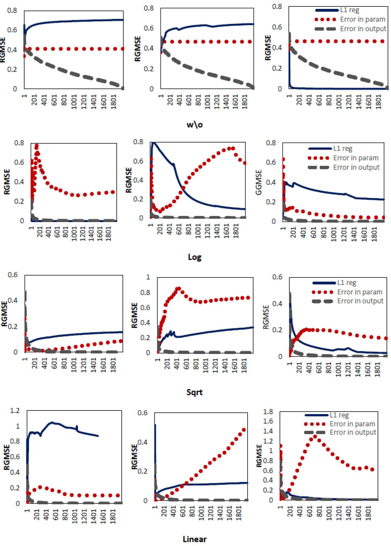
Comparison of RGMSE for different types of outliers; the share of the samples used in the training dataset:
Each row shows different types of outliers on the dataset: (w/o) original dataset without adding outliers (i.e., Log, Sqrt and Linear), where the number of outliers
Each column shows three different fraction of training dataset:
Table 2 (model
| k | BMM |
PBMM |
OBMM |
|||
|---|---|---|---|---|---|---|
| −1.1318 | 0.3898 | −2.4252 | 0.4315 | −1.1469 | 0.3962 | |
| −0.0339 | 0.0223 | −0.0819 | 0.0153 | −0.0343 | 0.0224 | |
| −0.0616 | 0.0385 | 0.0121 | 0.0324 | −0.0614 | 0.0386 | |
| 0.0186 | 0.4617 | 1.2399 | 0.3242 | 0.0285 | 0.4632 | |
| 0.1380 | 0.0491 | 0.2159 | 0.0457 | 0.1384 | 0.0490 | |
| −0.1279 | 0.0927 | 0.0399 | 0.0808 | −0.1278 | 0.0928 | |
| 1 | 0.2291 | 0.0818 | 0.3160 | 0.0704 | 0.2301 | 0.0817 |
| 2.0894 | 0.4519 | 4.6841 | 0.4094 | 2.1055 | 0.4628 | |
| −0.7119 | 0.6548 | −2.3642 | 0.5815 | −0.7503 | 0.6907 | |
| 0.1330 | 0.1288 | 0.3511 | 0.0894 | 0.1357 | 0.1307 | |
| −1.0179 | 0.3795 | −1.8398 | 0.3286 | −1.0262 | 0.3790 | |
| 0.2971 | 0.4797 | −1.0341 | 0.4926 | 0.2990 | 0.4802 | |
| −0.0016 | 0.0010 | −0.0034 | 0.0010 | −0.0016 | 0.0010 | |
| 0.0002 | 0.0009 | 0.0006 | 0.0002 | 0.0002 | 0.0009 | |
| 0.0113 | 0.3189 | −0.1207 | 0.3782 | 0.0113 | 0.3189 | |
| −0.0043 | 0.0148 | −0.0183 | 0.0177 | −0.0043 | 0.0148 | |
| −0.0023 | 0.0338 | 0.0392 | 0.0384 | −0.0023 | 0.0338 | |
| 0.0325 | 0.3526 | 1.0210 | 0.3784 | 0.0325 | 0.3526 | |
| 0.1339 | 0.0439 | 0.2152 | 0.0573 | 0.1339 | 0.0439 | |
| 0.1282 | 0.0820 | 0.4095 | 0.1049 | 0.1282 | 0.0820 | |
| 2 | 0.0108 | 0.0560 | −0.0293 | 0.0704 | 0.0108 | 0.0559 |
| 4.0875 | 0.4269 | 8.6061 | 0.8816 | 4.0875 | 0.4269 | |
| 1.2307 | 0.4384 | 1.0877 | 0.5550 | 1.2307 | 0.4384 | |
| 0.1042 | 0.0661 | 0.2849 | 0.1026 | 0.1043 | 0.0661 | |
| 0.16908 | 0.3102 | 0.1089 | 0.3531 | 0.1691 | 0.3102 | |
| −2.6615 | 0.4601 | −6.0474 | 0.7829 | −2.6615 | 0.4601 | |
| −0.0025 | 0.0012 | −0.0061 | 0.0013 | −0.0025 | 0.0012 | |
| 0.0009 | 0.0001 | 0.0019 | 0.0004 | 0.0009 | 0.0001 | |
BMM, Bernoulli mixture model; PBMM, parameter space in BMM.
Estimates and their standard deviations based on 2,000 runs on the original dataset without adding artificial outliers.
| k | BMM |
PBMM |
OBMM |
|||
|---|---|---|---|---|---|---|
| −1.2010 | 0.3741 | −1.4134 | 0.5099 | −1.2166 | 0.3770 | |
| −0.0370 | 0.0223 | −0.0447 | 0.0239 | −0.0376 | 0.0212 | |
| −0.0422 | 0.0362 | 0.0279 | 0.0386 | −0.0426 | 0.0349 | |
| 0.2765 | 0.4392 | 0.4722 | 0.4717 | 0.3072 | 0.4206 | |
| 0.1517 | 0.0462 | 0.1629 | 0.0511 | 0.1494 | 0.0466 | |
| −0.0574 | 0.0874 | 0.0323 | 0.0946 | −0.0527 | 0.0864 | |
| 1 | 0.1541 | 0.0756 | 0.1795 | 0.0852 | 0.1551 | 0.0730 |
| 2.2690 | 0.4286 | 2.6910 | 0.9504 | 2.2529 | 0.4337 | |
| −1.2131 | 0.5075 | −1.4257 | 0.4287 | −1.2208 | 0.4859 | |
| 0.2220 | 0.0651 | 0.2452 | 0.0737 | 0.2192 | 0.0658 | |
| −1.1937 | 0.3391 | −1.3085 | 0.3758 | −1.2083 | 0.3281 | |
| 0.0563 | 0.4798 | −0.1952 | 0.6393 | 0.0511 | 0.4619 | |
| −0.0028 | 0.0009 | −0.0029 | 0.0009 | −0.0028 | 0.0009 | |
| 0.0003 | 0.0001 | 0.0003 | 0.0002 | 0.0003 | 0.0001 | |
| 0.1157 | 0.3198 | −0.0833 | 0.3290 | 0.1096 | 0.3275 | |
| −0.0104 | 0.0148 | −0.0125 | 0.0160 | −0.0103 | 0.0144 | |
| −0.0090 | 0.0351 | 0.0135 | 0.0365 | −0.0062 | 0.0329 | |
| 0.2715 | 0.3605 | 1.4226 | 0.4718 | 0.2767 | 0.3599 | |
| 0.1379 | 0.0446 | 0.1502 | 0.0555 | 0.1362 | 0.0447 | |
| 0.2050 | 0.0837 | 0.2431 | 0.1198 | 0.2042 | 0.0822 | |
| 2 | 0.0534 | 0.0617 | −0.0488 | 0.0615 | −0.0521 | 0.0603 |
| 4.4087 | 0.4109 | 5.1751 | 1.8911 | 4.3724 | 0.3989 | |
| 0.9351 | 0.4350 | 0.9548 | 0.4725 | 0.9199 | 0.3903 | |
| 0.1620 | 0.0558 | 0.1816 | 0.0829 | 0.1592 | 0.0572 | |
| 0.1720 | 0.3284 | 0.1467 | 0.3258 | 0.1577 | 0.3027 | |
| −2.9528 | 0.4649 | −3.5070 | 1.4356 | −2.9171 | 0.4669 | |
| −0.0042 | 0.0011 | −0.0045 | 0.0013 | −0.0042 | 0.0010 | |
| 0.0010 | 0.0002 | 0.0012 | 0.0004 | 0.0010 | 0.0002 | |
| −0.2239 | 0.3374 | −0.2846 | 0.3565 | −0.2295 | 0.3403 | |
| −0.0021 | 0.0146 | −0.0033 | 0.0155 | −0.0019 | 0.0146 | |
| −0.0027 | 0.0347 | −0.0209 | 0.0365 | −0.0290 | 0.0335 | |
| 0.4231 | 0.3952 | 0.2910 | 0.4358 | 0.4132 | 0.3933 | |
| 0.1379 | 0.0491 | 0.1505 | 0.0570 | 0.1362 | 0.0492 | |
| −0.0482 | 0.0862 | −0.03477 | 0.0934 | −0.0488 | 0.0855 | |
| 3 | 0.2206 | 0.0773 | 0.2411 | 0.08556 | 0.2204 | 0.0755 |
| 4.0891 | 0.4534 | 4.7372 | 1.5019 | 4.0570 | 0.4535 | |
| 1.5783 | 0.4913 | 1.6599 | 0.5687 | 1.5755 | 0.4643 | |
| 0.0348 | 0.1026 | 0.0484 | 0.1032 | 0.0326 | 0.1033 | |
| 0.0196 | 0.3324 | 0.1495 | 0.3233 | 0.1865 | 0.3130 | |
| −2.1498 | 0.5279 | −2.6216 | 1.1565 | −2.1277 | 0.5287 | |
| −0.0001 | 0.0009 | −0.0001 | 0.0009 | −0.0001 | 0.0009 | |
| 0.0006 | 0.0002 | 0.0007 | 0.0003 | 0.0007 | 0.0002 | |
BMM, Bernoulli mixture model; PBMM, parameter space in BMM.
Estimates and their standard deviations based on 2,000 runs on the original dataset without adding artificial outliers.
5. DISCUSSION
In this paper, for the modeling sparsity of the outlier response vector on the BMMs, we randomly have selected a small number of
CONFLICTS OF INTEREST
The authors declare of no conflicts of interest.
AUTHORS' CONTRIBUTIONS
Prof. Eskandari with designed the model, idea and the computational framework and Mrs Sabbaghi analyzed the data. All authors discussed the results and contributed to the final manuscript.
ACKNOWLEDGMENTS
We would like to thank the editor and the referees for their valuable comments about our paper. This work is a part of my Ph.D Student thesis at Allameh Tabataba’i University.
REFERENCES
Cite this article
TY  - JOUR
AU  - Azam Sabbaghi
AU  - Farzad Eskandari
AU  - Hamid Reza Navabpoor
PY  - 2021
DA  - 2021/02/08
TI  - A Robust High-Dimensional Estimation of Multinomial Mixture Models
JO  - Journal of Statistical Theory and Applications
SP  - 21
EP  - 32
VL  - 20
IS  - 1
SN  - 2214-1766
UR  - https://doi.org/10.2991/jsta.d.210126.001
DO  - 10.2991/jsta.d.210126.001
ID  - Sabbaghi2021
ER  -