
Generalized Rank Mapped Transmuted Distribution for Generating Families of Continuous Distributions
- DOI
- 10.2991/jsta.d.210129.001How to use a DOI?
- Keywords
- Transmuted map; Order Statistics; Weibull distribution; Beta distribution; Hazard function; Continuous distributions
- Abstract
This study introduces generalized transmuted family of distributions. We investigate the special cases of our generalized transmuted distribution to match with some other generalization available in literature. The transmuted distributions are applied to Weibull distribution to find generalized rank map transmuted Weibull distribution. The distributional characteristics such as probability curve, mean, variance, skewness, kurtosis, distribution of largest order statistics, and their characteristics studied to compare with ordinary Weibull distribution. Hazard rate functions and distributional characteristics of largest order statistics of transmuted distributions are also studied. It is observed that the transmuted distributions are more flexible to model real data, since the data can present a high degree of skewness and kurtosis. If someone is interested to locate more flexible and higher degree of skewed distribution can explore this generalized transmuted family of distributions for future use.
- Copyright
- © 2021 The Authors. Published by Atlantis Press B.V.
- Open Access
- This is an open access article distributed under the CC BY-NC 4.0 license (http://creativecommons.org/licenses/by-nc/4.0/).
1. INTRODUCTION
The ideas of developing new distributions are important issues in recent literatures. Numerous families of distributions have proposed by several authors for modeling data in several areas such as engineering, economics, finance and actuarial science, medical and life sciences. However, in many applied areas like lifetime analysis, insurance analysis we need extended distributions, that is, new distributions which are more flexible to model real data, since the data can present a high degree of skewness and kurtosis.
Lee et al. [1] provided an overview of most method used to generate family of continuous distributions earlier in 1980. For more details about these methods can be referred to Pearson [2], Johnson [3], and Tukey [4]. Recently several literatures were discussed generalized method to generate extended generalized family of distributions. For more details about the recent development may refer to Johnson et al. [5], Eugene et al. [6], Jones [7], Alzaatreh et al. [8], Bourguignon et al. [9], Afify et al. [10], Granzotto et al. [11], Al-Kadim and Mohammed [12], Jayakumar and Babu [13], Mahdavi and Kundu [14], Alizadeh et al. [15], Al-Kadim [16], Pobocikova et al. [17], Elgarhy et al. [18], Afify et al. [19], and references therein. Apart from the above, a more extended generalized nth degree transmuted method suggested in this study to generate transmuted distributions. An application of the generated transmuted map is extended to the Weibull distribution. The distributional characteristics of the generated transmuted distributions are also simulated to compare with traditional Weibull distribution.
This paper is organized in the following way: In Section 2, we developed nth degree generalized transmutation map based on continuous family of distribution. Particular cases are also discussed. Some other members of generalized transmutation map are identified. In Section 3, the survival function, hazard rate function, and reserved hazard rate function of newly generated generalized transmuted distribution are discussed. In Section 4, we developed the nth degree generalized transmutation map based on Weibull distribution. Also, probability density function (pdf) graphs are simulated and presented in figure to compare each other. In Section 5, some distributional characteristics such as mean variance, skewness, and kurtosis are simulated and presented in tabular form to compare each other for different parametric set of values. The Section 6 is based on discussion and proof of some theorems related to order statistics (OS) of generalized transmuted Weibull distribution (TWD). Simulated distributional characteristics of largest OS of quadratic TWD are also presented in section 6. The Section 7, states conclusion and then inserted references.
2. GENERALIZED nth RANK TRANSMUTATION MAP
The construction of the generalized n-degree transmutation map considered here is simple and intuitive. Let
The equalities
As
Let
Now, consider the random variable,
where
Hence, generalized transmuted cdf of nth rank mapped (n = 1, 2, 3, …) distribution is given by
Now,
Expression (3) and (7) will also be helpful for simulation study for the cdf and pdf respectively.
2.1. Particular Cases
Put
and the corresponding pdf of quadratic transmutation map of Shaw and Buckley [20] isPut
and the pdf of cubic ranking transmutation map of Granzotto et al. [11] isPut
and the pdf of simple transmutation map of Eugene et al. [6] isPut
and the corresponding pdf of the cubic ranking transmutation map of Al-Kadim and Mohammed [12] isIt may be noted that the general formula of the transmuted distribution of Al-Kadim [16] can also be deduced from (3) as a particular case for odd and even n respectively.
Put
and the corresponding generalized Quartic ranking transmutation map with new pdf as suggested is given byPut
and the corresponding pdf of generalized Quintic ranking transmutation map which is a new pdf as suggested isPut
If one put,
If we put,
wherewhere,
Some Specific Cases of (12) and (13)
2.1.1. Quadratic rank transmuted distribution (TD2)
For n = 2 in (12) and (13), the new form of quadratic map ranked transmuted cdf is given by
2.1.2. Cubic rank transmuted distribution (TD3)
For n = 3 in (12) and (13), the new form of cubic ranked transmuted cdf is given by
2.1.3. Quartic rank transmuted distribution (TD4)
For n = 4 in (12) and (13), the new form of quartic ranked transmuted cdf is given by
2.1.4. Quintic rank transmuted distribution (TD5)
For n = 5 in (12) and (13), the new form of quintic ranked transmuted cdf is given by
In a similar manner, one can generate any desired higher order
3. HAZARD FUNCTION
The survival function
Use (3) in (22) to get survival function for newly derived nth ranked transmuted distribution as
Use (7) and (22) in (23) to get hazard rate function for newly derived nth ranked transmuted distribution as
Use (3) and (7) in (24) to get reserved hazard rate function for newly derived nth ranked transmuted distribution as
For more about the hazard function one can refer to Zubair et al. [21] and references therein.
Theorem 3.1.
The quadratic generalized transmuted hazard rate function is given by
Proof.
From (23) and for n = 2, we get the generalized transmuted hazard rate function as
Now using (14) and (15) in (28) and on algebraic simplification gives the proof of the theorem.
Theorem 3.2.
The quadratic generalized transmuted Weibull hazard rate function is given by
Proof.
From (28) and on using (29) and (30) gives the proof of the theorem.
Simulated hazard function (WD, TWD2 to TWD5) for some specific sets of parameters (α, β) values are presented in Figures 1–4 to compare among themselves. The hazard function is one of the most important quantities to character life phenomenon. Compare with many other modified Weibull distributions, the shape of the hazard function is easy to decide. It can be derived from (23) and it is flexible. As we know, it is very common for a bathtub-shaped hazard function of a system or component to have a long useful lifetime with low constant rate portion in the middle and sharp change in the initial and wear-out of phase, so a distribution which can fit this kind of hazard rate would be very useful in reliability studies.
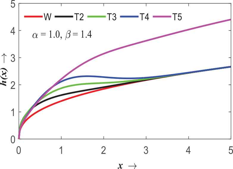
Hazard rate curve for
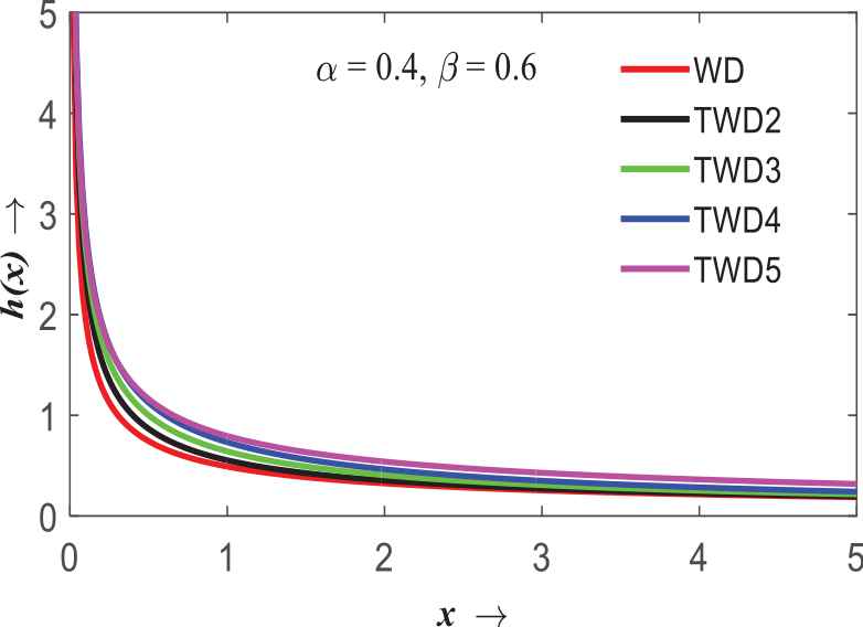
Hazard rate curve for
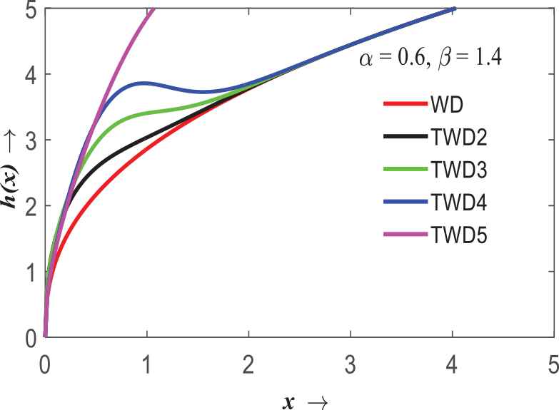
Hazard rate curve for
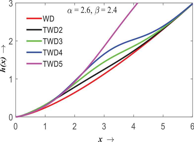
Hazard rate curve for
4. TRANSMUTED WEIBULL DISTRIBUTION
The Weibull distribution which was proposed by Weibull [22] is a very important lifetime distribution and is widely used in many fields. However, the hazard function of the traditional Weibull distribution can only be increasing, decreasing, or constant. To meet the need of fitting complex modes and the bathtub-shaped hazard rate, researchers have proposed many improved flexible models based on the traditional Weibull distribution. To know more about modified or improved models based on the traditional Weibull distribution, one may refer to Johnson et al. [5], Xie et al. [23], Bebbington et al. [24], Nassar et al. [25], Afify et al. [19], and references therein. Still even available modified Weibull model are not enough to represent or fit the data obtain all cases such as engineering, economics, finance and actuarial science, medical and life sciences. Our proposed transmuted model will be more flexible and will cover such limitation for which data present a higher degree of skewness and kurtosis.
A random variable X is said to have traditional Weibull distribution (WD) with parameters
Quadratic ranked map Transmuted Weibull distribution (TWD2)
Using (29) in (14); (29) and (30) into (15) to get the new Quadratic map ranked transmuted Weibull cdf as
and the corresponding new Quadratic map ranked transmuted Weibull pdf is given byCubic ranked map Transmuted Weibull distribution (TWD3)
Using (29) in to (16); (29) and (30) into (17) to get the new Cubic map ranked transmuted Weibull cdf as
and the corresponding new cubic map ranked transmuted Weibull pdf is given byQuartic ranked map Transmuted Weibull distribution (TWD4)
Using (29) in to (18); (29) and (30) into (19) to get the new Quartic map ranked transmuted Weibull cdf as
and the corresponding new Quartic ranked transmuted Weibull pdf is given byQuintic ranked map Transmuted Weibull distribution (TWD5)
Using (29) in to (20); (29) and (30) into (21) to get new the Quartic map ranked transmuted Weibull cdf as
and the corresponding new quartic ranked transmuted Weibull pdf is given by
In a similar way one can find new any desired rank map transmuted cdf of Weibull distribution by using (29) in to (12); corresponding pdf by using (29) and (30) into (13).
The simulated pdf curves of different ranked TWD for some specific sets of parametric values (α, β) were plotted in Figures 5–8 to observe and compare the change of skewness and the pdf curve shapes with the change of transmutation rank.
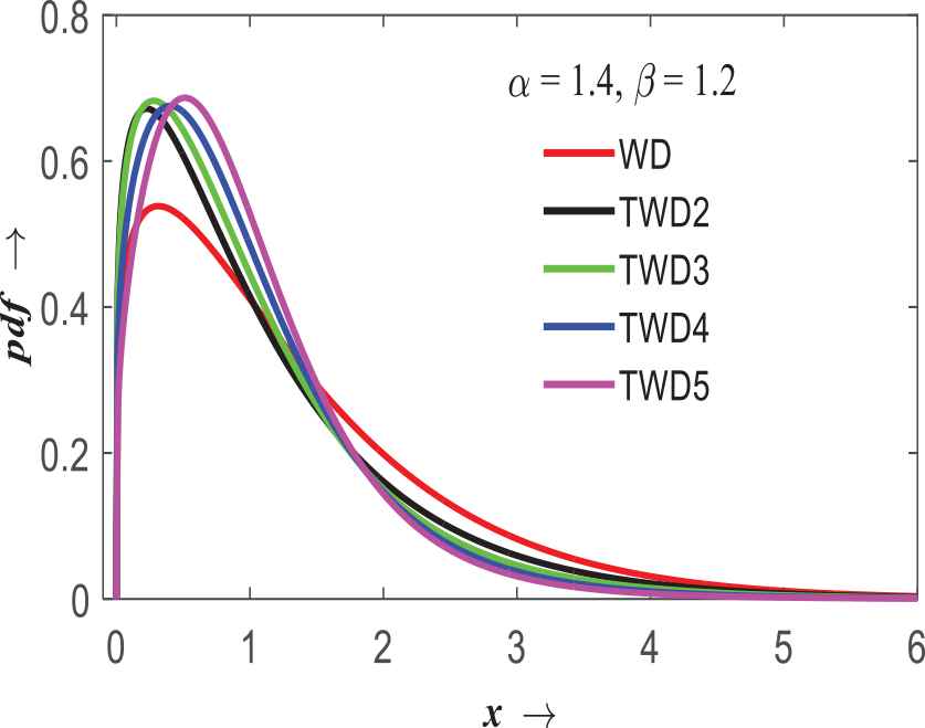
TWDn curve for
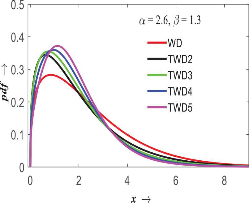
TWDn curve for
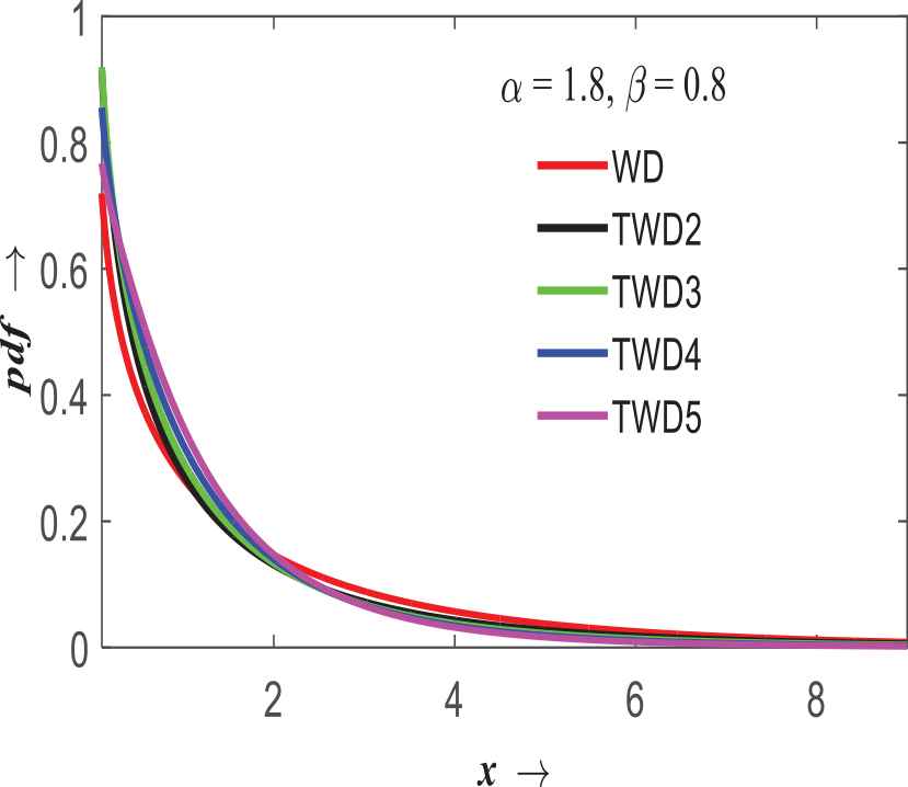
TWDn curve for
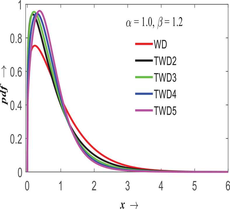
TWDn curve for
It is observed from the above Figures 5–8 that the TWDs are more skewed compare to ordinary Weibull distribution. The degree of skewness of TWDn curves increases if the rank of transmutation map increases. So, the newly generated TWDs have advantages to fit if the data sets are more skewed.
5. DISTRIBUTIONAL CHARACTERISTICS
The kth (
Now on using (29) and (30), we have
We know that
5.1. Moments for Quadratic TWD2
For n = 2 in (39), the kth raw moment of the quadratic TWD is given by
The central moments are given by
Pearson's four coefficients, based upon the first four central moments are
It may be noted that these coefficients are true numbers independent of units of measurement.
The pth
5.2. Moments for Cubic TWD3
For n = 3 in (39), the kth raw moment of the Cubic TWD is given by
From (34), the rth raw moment of TWD3 is given by
Other central moments and Pearson's four coefficients can be obtained from the above by simple algebraic manipulation.
5.3. Moments for Quartic TWD4
For n = 4 in (39), the kth raw moment of the TWD4 is given by
5.4. Moments for Quintic TWD5
For n = 5 in (39), the kth raw moment of the TWD5 is given by
For example, some distributional properties like mean, variance, skewness, and kurtosis are simulated and presented below in Table 1 for some specific values of the parameters (α, β) to observe and compare differentiation of traditional Weibull distribution (30) along with some other different ranked map TWD (TWDn, n = 2,3, 4, 5), where, n indicates nth rank (31–38) map. It is observed that skewness of transmuted distribution is more flexible as rank of transmutation increases. So, one can use flexible desired rank map transmuted distribution to fit desired skewed data set. For all simulation work MATLAB R2015a version is used.
| Distributional Characteristics | Different Combination of Parameter (α, β) Values |
||||||||||
|---|---|---|---|---|---|---|---|---|---|---|---|
| Means | WD | 0.9970 | 1.0000 | 1.1083 | 1.0937 | 1.1736 | 1.0833 | 0.6000 | 0.2659 | 1.9559 | 0.2000 |
| TWD2 | 0.7566 | 1.0000 | 1.1714 | 1.1714 | 1.2715 | 1.1737 | 0.4886 | 0.2998 | 1.6909 | 0.1629 | |
| TWD3 | 0.5841 | 0.8988 | 1.0684 | 1.0717 | 1.1662 | 1.0765 | 0.3993 | 0.2771 | 1.4330 | 0.1331 | |
| TWD4 | 0.4571 | 0.7511 | 0.8879 | 0.8890 | 0.9658 | 0.8915 | 0.3255 | 0.2280 | 1.1889 | 0.1085 | |
| TWD5 | 0.3654 | 0.6025 | 0.6980 | 0.6951 | 0.7515 | 0.6936 | 0.2673 | 0.1743 | 0.9806 | 0.0891 | |
| Variances | WD | 9.8060 | 1.0000 | 0.7391 | 0.6266 | 0.6349 | 0.5410 | 1.8000 | 0.0193 | 11.8246 | 0.2000 |
| TWD2 | 6.6876 | 0.6287 | 0.3727 | 0.2819 | 0.2473 | 0.2107 | 1.2411 | 0.0001 | 8.1840 | 0.1379 | |
| TWD3 | 4.4160 | 0.5232 | 0.3566 | 0.2867 | 0.2715 | 0.2314 | 0.8456 | 0.0041 | 5.7940 | 0.0940 | |
| TWD4 | 2.8471 | 0.5209 | 0.4601 | 0.4087 | 0.4322 | 0.3683 | 0.5756 | 0.0156 | 4.2317 | 0.0640 | |
| TWD5 | 1.7331 | 0.3269 | 0.2397 | 0.1943 | 0.1842 | 0.1570 | 0.3615 | 0.0022 | 2.7453 | 0.0402 | |
| Skewness | WD | 142644.2686 | 35.0000 | 21.4433 | 15.4247 | 19.0513 | 11.7856 | 372.0816 | 0.0013 | 67852.7372 | 0.5104 |
| TWD2 | 63555.1105 | 18.5292 | 13.1605 | 9.9132 | 12.7894 | 7.9119 | 166.8259 | 0.0010 | 30860.4307 | 0.2288 | |
| TWD3 | 26345.0289 | 9.9275 | 8.1805 | 6.4000 | 8.5316 | 5.2779 | 69.9412 | 0.0008 | 13291.0082 | 0.0959 | |
| TWD4 | 10238.2132 | 5.4371 | 5.1186 | 4.1148 | 5.6021 | 3.4656 | 27.6680 | 0.0005 | 5489.6068 | 0.0380 | |
| TWD5 | 3764.5469 | 3.2185 | 3.4063 | 2.7832 | 3.8259 | 2.3668 | 10.4650 | 0.0004 | 2226.7486 | 0.0144 | |
| Kurtosis | WD | 305.6793 | 24.0000 | 25.1054 | 26.5616 | 28.4265 | 28.4265 | 100.8000 | 43.4273 | 52.9786 | 100.8000 |
| TWD2 | 438.1475 | 41.5948 | 70.8843 | 95.9613 | 139.5531 | 139.5531 | 141.3656 | 741.4459 | 73.7997 | 141.3656 | |
| TWD3 | 645.9979 | 40.8002 | 56.3043 | 68.9036 | 87.7369 | 87.7369 | 195.8565 | 642.8510 | 94.8898 | 195.8565 | |
| TWD4 | 967.0436 | 27.9066 | 24.9716 | 25.6054 | 26.6692 | 26.6692 | 263.1634 | 36.1091 | 111.1517 | 263.1634 | |
| TWD5 | 1578.6245 | 48.6008 | 69.6797 | 87.7467 | 115.7325 | 115.7325 | 404.0340 | 455.9642 | 160.7934 | 404.0340 | |
Distributional characteristics of
6. ORDER STATISTICS
OS and functions of OS play an important role in statistical theory and methodology. Floods and droughts, longevity, breaking strength, aeronautics, oceanography, duration of humans, organisms, components, and devices of various kinds can be studied by the theory extreme values. Life tests provide an ideal illustration of the advantage of OS in censored data. Since such an experiment may take a long time to complete, it is often advantageous to stop after failure of the first r out of n similar items under test. For more details and development of OS one may refer to Sarhan and Greenberg [27], Arnold and Balakrishnan [28], Balakrishnan and Cohen [29], Arnold et al. [30], Ali [31], and David and Nagaraja [32].
The pdf of
The pdf of extreme OS follows from (45) at r = 1 and r = n respectively given by
Theorem 6.1.
For
Proof.
From (47) and on using (14) and (15), we have
Now using
Theorem 6.2.
For
Proof.
Multiplying both sides of (48) by
Theorem 6.3.
For
Proof.
We know that
Now using this result in (48) and on algebraic manipulation, we get the required result.
Theorem 6.4.
For
Proof.
For Weibull distribution defined in (29) and (30), we have
By expanding above expression binomially, we get
Now kth order moment of largest OS of Weibull distribution (30) is given by
Since
Therefore,
Now using (53) in (49) for
Now on algebraic manipulation, we have
Hence the theorem.
7. CONCLUSIONS
In this paper we have generated new generalized transmuted family of distributions (TDn). Some generalized transmuted distributions available in literature are found as particular cases of our transmuted family of distributions. These new generalized transmuted families of distributions are applied to Weibull distribution to find generalized rank map transmuted Weibull distribution (TWDn). Simulated hazard function, pdf curves, and some distributional characteristics such as mean, variance, skewness, and kurtosis for some specific parametric values of generalized transmuted families of Weibull distribution are presented in Figures 1–8 and in Table 1 respectively to make a comparative study among changes of rank maps. Also simulated quadratic ranked transmuted largest os's distributional characteristics are studied and presented in Table 2. These new distributions are more flexible and skewed compare to ordinary Weibull distribution. Flexibility prominently increases as degree of rank of transmutation map increases. These are observed in pdf curves (Figure 4–8) plotting as well as in distributional characteristics presented in Table 1. It is observed that the transmuted distributions are more flexible to model real data, since the data can present a high degree of skewness and kurtosis. If someone is interested to locate more flexible and higher degree of skewed distribution can explore this generalized transmuted family of distributions for future use.
| n | ||||||||||||
|---|---|---|---|---|---|---|---|---|---|---|---|---|
| Mean | Var | Skew | Kurto | Mean | Var | Skew | Kurto | Mean | Var | Skew | Kurto | |
| 2 | 0.2533 | 0.3362 | 1.2027 | 1.8339 | 2.0547 | 23.3801 | 25.5977 | 56.0054 | 0.8056 | 3.9894 | 1.4560 | 1.8314 |
| 3 | 0.3605 | 0.4288 | 0.3614 | 1.0651 | 2.8803 | 32.3545 | 18.0286 | 41.2666 | 1.1767 | 5.1747 | 0.4353 | 0.9362 |
| 4 | 0.4428 | 0.4923 | 0.0961 | 0.8081 | 3.6262 | 40.2543 | 14.0814 | 33.6843 | 1.4542 | 5.9506 | 0.1244 | 0.6501 |
| 5 | 0.5112 | 0.5401 | 0.0097 | 0.7112 | 4.3217 | 47.2606 | 11.6460 | 29.0873 | 1.6804 | 6.5160 | 0.0184 | 0.5415 |
| 6 | 0.5708 | 0.5779 | 0.0053 | 0.6877 | 4.9808 | 53.4868 | 9.9987 | 26.0429 | 1.8741 | 6.9525 | 0.0013 | 0.5097 |
| 7 | 0.6242 | 0.6084 | 0.0482 | 0.7061 | 5.6114 | 59.0147 | 8.8196 | 23.9196 | 2.0454 | 7.3006 | 0.0325 | 0.5195 |
| 8 | 0.6731 | 0.6334 | 0.1233 | 0.7526 | 6.2186 | 63.9072 | 7.9448 | 22.3947 | 2.2003 | 7.5835 | 0.0946 | 0.5553 |
| 9 | 0.7184 | 0.6539 | 0.2231 | 0.8201 | 6.8060 | 68.2150 | 7.2812 | 21.2858 | 2.3425 | 7.8156 | 0.1789 | 0.6095 |
| 10 | 0.7608 | 0.6706 | 0.3435 | 0.9048 | 7.3763 | 71.9799 | 6.7727 | 20.4830 | 2.4746 | 8.0067 | 0.2807 | 0.6779 |
Distributional characteristics of largest OS of TWD2 (48) for different parametric values and sample size.
CONFLICT OF INTEREST
The authors declare that there are no conflicts of interest regarding the publication of this paper.
AUTHORS' CONTRIBUTIONS
All authors have read and agreed to the published version of the manuscript.
ACKNOWLEDGMENTS
The author would like to thank the Editor-in-Chief, and the anonymous referees for their careful reading and constructive comments and suggestions which greatly improved the presentation of the paper.
REFERENCES
Cite this article
TY  - JOUR
AU  - M. A. Ali
AU  - Haseeb Athar
PY  - 2021
DA  - 2021/02/05
TI  - Generalized Rank Mapped Transmuted Distribution for Generating Families of Continuous Distributions
JO  - Journal of Statistical Theory and Applications
SP  - 132
EP  - 148
VL  - 20
IS  - 1
SN  - 2214-1766
UR  - https://doi.org/10.2991/jsta.d.210129.001
DO  - 10.2991/jsta.d.210129.001
ID  - Ali2021
ER  -