
Bayesian Estimation of System Reliability Models Using Monte-Carlo Technique of Simulation
- DOI
- 10.2991/jsta.d.210201.001How to use a DOI?
- Keywords
- Bayesian estimation; Bayes Estimator; Reliability; Monte-Carlo simulation
- Abstract
This paper discusses the problem of how Monte-Carlo simulation method is deal with Bayesian estimation of reliability of system of n s-independent two-state component. Time-to-failure for each component is assumed to have Weibull distribution with different parameters for each component. The shape parameter for each component is assumed to be known with the scale parameter distributed with a priori Rayleigh distribution with known parameters. Monte-Carlo simulation is used to generate the random deviates for the scale parameters and replicates for time-to-failure for each combination of scale parameters values are generated. Reliability is estimated as a function of time. Further, for the Bayes estimation of reliability we assume Poisson distribution with a priori time-shifted Rayleigh distribution. Finally, the robustness in the Bayesian estimation problem relative to changes in the assigned priori distribution is considered. We approximate the Bayes estimator of the reliability. The Bayes risk with respect to the priori time-shifted beta distribution is considered and at last approximate robustness of the Bayes estimator of reliability is examined with respect to the uniform priori. We have compared the maximum likelihood estimator of reliability with the Bayes estimator with prior uniform distribution. Finally, the method is illustrated by considering the illustrative example of vehicle system.
- Copyright
- © 2021 The Authors. Published by Atlantis Press B.V.
- Open Access
- This is an open access article distributed under the CC BY-NC 4.0 license (http://creativecommons.org/licenses/by-nc/4.0/).
1. INTRODUCTION
Bayesian estimation modelling is used for system identification, prediction and performance of reliability of the model. Bayesian inference requires the numerical approximation of the posteriors. Monte Carlo sampling is used for Bayesian Calculation. Modelling updating is used to improve the accuracy of predications of the reliability system (Bhattacharya [1], Box and Tiao [2−4]). Some researchers had introduced the two parameter generalization of Lindley distribution as a prolonged model of bathtub data alternative gamma, lognormal, Weibull, and exponential distribution. (Beck and Katafygiotis [5], Beck [6], Papadimitriou et al. [7], Nadarajah et al. [8]). Recently Wilson and Huzurbazar [9] had worked on the systems reliability. He had used the Bayesian networks for it. This model had binary outcomes and discrete data as multilevel form. Singh et al. [10] had used the generalized Lindley distribution under squared error and general entropy loss functions to develop the Bayesian estimation procedure in case f complete sample of observations. The estimating the reliability of a network through variations of Monte Carlo simulation is one of the active area for research [11–15].
In the present paper, Monte-Carlo simulation method is applied for Bayesian estimation of reliability of system of n s-independent two state components. Time-to-failure for each component is assumed to have Weibull distribution with different parameters for each component. The shape parameter for each component is assumed to be known with the scale parameter distributed with a priori Rayleigh distribution with known parameters. Monte-Carlo simulation is used to generate to generate the random deviates for the scale parameters and replicates for time-to-failure for each combination of scale parameters values are generated. Reliability is estimated as a function of time. Further, for the Bayes estimation of reliability we assume Poisson distribution with a priori time-shifted Rayleigh distribution. Finally, the robustness in the Bayesian estimation problem relative to changes in the assigned priori distribution is considered. We approximate the Bayes estimator of the Reliability. The Bayes risk with respect to the priori time-shifted beta distribution is considered and at last approximate robustness of the Bayes estimator of reliability is examined with respect to the Uniform priori. We have compared the maximum likelihood estimator of reliability with the Bayes estimator with prior Uniform Distribution.
2. ROBUSTNESS AND TIME-SHIFTED BETA PRIORI DISTRIBUTION IN THE BAYESIAN ESTIMATION
Consider the Rayleigh distribution with probability density function (pdf),
Let the reliability at time t be defined as the probability of zero failures occurring at time t, thus,
The likelihood function is
The uniform minimum variance unbiased estimator (MVUE) of reliability is
Suppose that the intensity parameter
Let,
Where
Hence, the relation
Similarly, the posterior variance is evaluated to be
Since, the Bayes risk is defined as the expectation of the posterior variance where expectation is taken over all possible random variables. Thus,
Now, with the help of Equation (7), Equation (8) can be written as
Now by taking expectation with respect K, for the priori distribution,
3. ROBUSTNESS BY RAYLEIGH DISTRIBUTION IN THE BAYESIAN ESTIMATION
The robustness of the Bayes estimator,
In the determination of the risk, we note that Equation (8) is the result before taking expectations with respect to
Finally, for comparison the MLE of reliability over the uniform distribution is given by,
For numerical comparison, two ratios are formed and computed for various values of the indicated parameters. The first involves the ratio of the Bayes risk
| x = 5, xw = 2, K = 3, s = 10 |
||||||
|---|---|---|---|---|---|---|
| T | µ = 3.5, |
µ = 3.5, |
||||
| 1 | 1.5 | 3.5 | 2.765 | 1.5 | 3.5 | 0.172 |
| 2 | 1.5 | 4.5 | 3.555 | 1.5 | 4.5 | 0.222 |
| 3 | 1.5 | 5.5 | 4.345 | 1.5 | 5.5 | 0.271 |
| 4 | 1.5 | 6.5 | 5.135 | 1.5 | 6.5 | 0.320 |
| 5 | 1.5 | 7.5 | 5.925 | 1.5 | 7.5 | 0.370 |
| 6 | 1.5 | 8.5 | 6.716 | 1.5 | 8.5 | 0.419 |
| 7 | 1.5 | 9.5 | 7.506 | 1.5 | 9.5 | 0.469 |
| 8 | 1.5 | 10.5 | 8.296 | 1.5 | 10.5 | 0.518 |
| 9 | 1.5 | 11.5 | 9.086 | 1.5 | 11.5 | 0.567 |
| 10 | 1.5 | 12.5 | 7.601 | 1.5 | 12.5 | 0.475 |
Ratio of
| x = 5, xw = 2, K = 3, s = 10 |
||||||
|---|---|---|---|---|---|---|
| T | µ = 3.5, |
µ = 3.5, |
||||
| 1 | 1.0 | 2.0 | 0.343 | 1.0 | 2.0 | 1.72 |
| 2 | 1.0 | 2.5 | 0.309 | 1.0 | 2.5 | 1.45 |
| 3 | 1.0 | 3.0 | 0.251 | 1.0 | 3.0 | 1.15 |
| 4 | 1.0 | 3.5 | 0.194 | 1.0 | 3.5 | 0.85 |
| 5 | 1.0 | 4.0 | 0.143 | 1.0 | 4.0 | 0.60 |
| 6 | 1.0 | 4.5 | 0.101 | 1.0 | 4.5 | 0.41 |
| 7 | 1.0 | 5.0 | 0.092 | 1.0 | 5.0 | 0.36 |
| 8 | 1.0 | 5.5 | 0.026 | 1.0 | 5.5 | 0.31 |
| 9 | 1.0 | 6.0 | 0.076 | 1.0 | 6.0 | 0.27 |
| 10 | 1.0 | 6.5 | 0.068 | 1.0 | 6.5 | 3.60 |
Ratio of
3.1. Illustrate Example on Vehicle System Model Based on Above Results
The model for the system of vehicles, that is, all the passenger carrying vehicles in the system. The model is based on the following assumptions:
Only the operating vehicles are liable to fail and the vehicles on standby or maintenance are not subject to failure. This assumption results in assigning zero failure rates to the vehicles being maintained or in standby mode. The failure rate of a cold standby mode, that is, partially powered, this assumption is valid only so long as the failure rate in warm standby mode is small as compared with that of the operating vehicle.
The failure of a single vehicle in the retrieval mode causes the whole system of vehicles to be down. The duration of the down time of a vehicle is considered from the time it comes to a halt to time of resuming normal operation. The down time of all the vehicles, directly affected vehicle, and the vehicles coming to a halt as a result of blocking, is assumed to be the same. This assumption was made because of short headways, all the vehicles may not be equally affected and a correction to models may be needed.
A vehicle in a partial failure mode is assumed to be removed from the system as soon as possible after the occurrence of the failure and therefore the probability of another unit failing during this period or the partial mode passing into full mode is assumed zero.
So long as there one standby, a unit on which maintenance is completed will be interchanged with an operating or standby unit. When, however, no spares are left, the unit passes directly from maintenance into the operation mode, without going on standby.
Now, we illustrate the example based on the above model.
3.2. Vehicle System Example
The model described above has been implemented in a computer program.
The vehicle system data for this example is described in the above. The system consists of 12 vehicles out of which one are on maintenance and one kept as spares.
3.3. Vehicle System Data
Time to vehicle failure (permanent)
Wear-out time to vehicle failure (partial mode)
Number of operating vehicle
Number of spare vehicle
Number of vehicle on maintenance
Vehicle exposure factor
Now, we construct the Table 3, for the comparison two ratios.
| t (No of vehicles) | µ = 1.0, |
||||
|---|---|---|---|---|---|
| 1 | 1.0 | 0.001 | 6.1262 | 980.198 | 6.420 |
| 2 | 5.9495 | 951.923 | 10.912 | ||
| 3 | 5.6766 | 908.256 | 16.487 | ||
| 4 | 5.3340 | 853.448 | 23.353 | ||
| 5 | 4.9499 | 791.999 | 31.755 | ||
| 6 | 4.5496 | 727.941 | 41.980 | ||
| 7 | 4.1526 | 664.429 | 54.365 | ||
| 8 | 3.7728 | 603.658 | 69.304 | ||
| 9 | 3.4185 | 546.961 | 87.258 | ||
| 10 | 3.0937 | 494.999 | 108.764 | ||
Ratio of
3.4. Concluding Remarks
It is apparent from these results that when the perturbed risk
4. BAYESIAN ESTIMATION OF RELIABILITY WITH PRIORI TIME-SHIFTED RAYLEIGH DISTRIBUTION USING MONTE-CARLO SIMULATION
Consider the Poisson distribution, with parameter ‘a’ and probability mass function (pmf),
The MVUE of reliability is
While the mean-squared error (MSE) of
Suppose that the intensity parameter ‘a’ is a random variable. Assume the time-shifted Rayleigh distribution as the priori distribution of “a” with probability distribution function is
Since, the relation
4.1. Monte-Carlo Simulation
To establish the usefulness of the Bayes estimators of reliability Monte-Carlo simulation is employed. There exist point epochs at which stochastic process regenerates itself and makes the future evaluation of the process conditionally independent of the past manners. This is an important possession, which is used in simulation experiments regarding the behavior of the system.
The procedure available for the generation of random deviations useful in reliability theory. The central concept is the generation of random numbers of a uniform random variable on (0, 1). By using the computer program, the random deviates for the arbitrary values of the parameters are generated. Further, the reliability for Weibull and negative exponential distributions for lifetime is calculated which is shown in Table 3. The importance of uniformly distributed variables for Weibull and negative exponential distributions is clear from the following results.
Let X be a random variable with pdf, fX(.) and cumulative distribution
The new random variable
5. BAYESIAN ESTIMATION OF RELIABILITY WITH NEGATIVE EXPONENTIAL DISTRIBUTION USING MONTE-CARLO SIMULATION
Let T be a negative exponentially distributed random variable with pdf
| Weibull Distribution | Negative Exponential Distribution | |||||
|---|---|---|---|---|---|---|
| a = b = 5.0 | a = b = 10.0 | |||||
| U | T | Bayes Reliability |
U | T | Bayes Reliability |
|
| 0.6459 | 3.5862 | 0.9874 | 0.9711 | 2.0891 | 0.8615 | |
| 0.1957 | 4.6688 | 0.8546 | 0.9564 | 2.2717 | 0.7451 | |
| 0.1993 | 4.6564 | 0.8052 | 0.9345 | 2.4700 | 0.6321 | |
| 0.1635 | 4.7654 | 0.7456 | 0.7038 | 3.4328 | 0.5211 | |
| 0.0794 | 5.0963 | 0.6542 | 0.7025 | 3.4364 | 0.5016 | |
| 0.0623 | 5.1904 | 0.5321 | 0.6712 | 3.5208 | 0.4123 | |
| 0.0616 | 5.1946 | 0.5021 | 0.5644 | 3.7844 | 0.3014 | |
| 0.0022 | 6.0794 | 0.4562 | 0.5349 | 0.8529 | 0.2015 | |
| 0.0010 | 6.2286 | 0.3154 | 0.5318 | 0.8601 | 0.1206 | |
| 0.0004 | 6.3857 | 0.2154 | 0.3209 | 4.3416 | 0.1123 | |
Monte-Carlo simulation result.
6. BAYESIAN ESTIMATION OF RELIABILITY WITH WEIBULL DISTRIBUTION USING MONTE-CARLO SIMULATION
Let T be a Weibull distribution with pdf
The cdf of T denoted as
To generate T, generate the uniform variable U, and using relation (21). Thus, we generate the random number from uniform variable in (0, 1) and using Equation (21). We assume some erratic values of the parameters and assess the T, which is shown in Table 4. Then the curves are plotted for the above values obtained in Table 4.
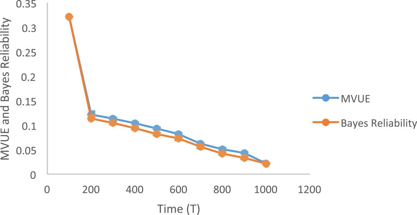
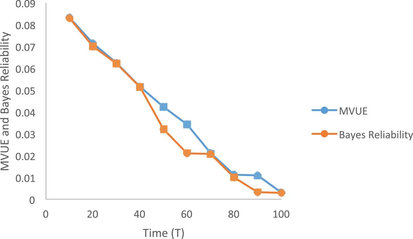
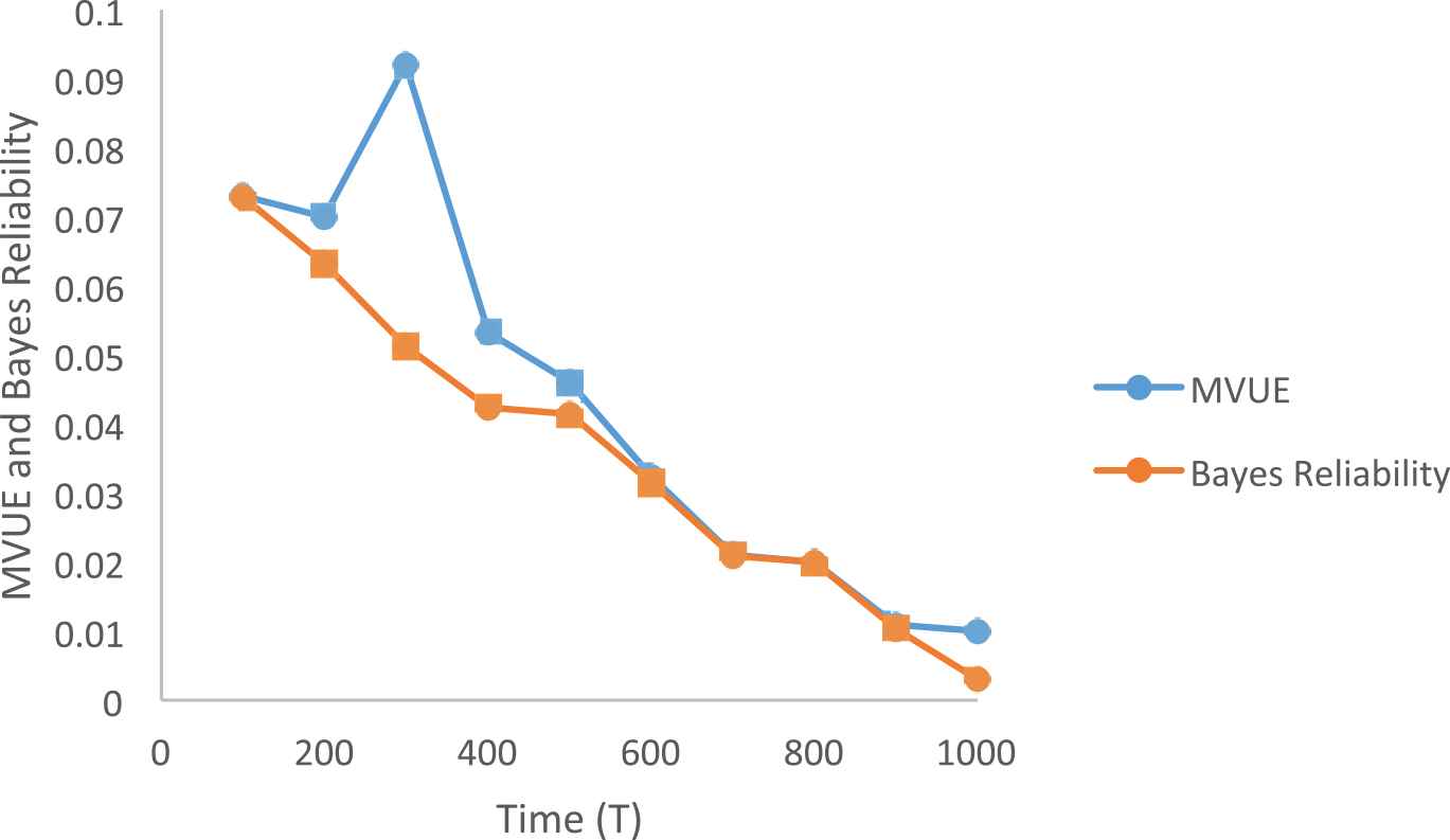
Then subsequently the Table 5, represents the values of the MVUE and Bayes reliability for the different values of T. Furthermore, the curves for the MSE, minimum unbiased estimator (MVUE), and Bayes reliability are drawn to show the fluctuations. This is useful for the system designers or engineers to design more reliable systems.
| Negative Exponential Distribution |
||||||||
|---|---|---|---|---|---|---|---|---|
| ts = 100; a = 2.0; |
ts = 1000; a = 2.0; |
|||||||
| T | MSE | MVUE | Bayes Reliability | T | MSE | MVUE | Bayes Reliability | |
| 10 | 0.0295 | 0.5213 | 0.3216 | 100 | 0.0318 | 0.3216 | 0.3212 | |
| 20 | 0.0288 | 0.4021 | 0.3116 | 200 | 0.1216 | 0.1216 | 0.1134 | |
| 30 | 0.0224 | 0.4011 | 0.3016 | 300 | 0.1132 | 0.1132 | 0.1046 | |
| 40 | 0.0202 | 0.3412 | 0.2664 | 400 | 0.1042 | 0.1042 | 0.0936 | |
| 50 | 0.0065 | 0.2316 | 0.1334 | 500 | 0.0932 | 0.0932 | 0.0819 | |
| 60 | 0.0033 | 0.2033 | 0.1942 | 600 | 0.0816 | 0.0816 | 0.0732 | |
| 70 | 0.0077 | 0.1666 | 0.1389 | 700 | 0.0621 | 0.0621 | 0.0561 | |
| 80 | 0.0015 | 0.1232 | 0.1124 | 800 | 0.0511 | 0.0511 | 0.0421 | |
| 90 | 0.0200 | 0.1200 | 0.1020 | 900 | 0.0432 | 0.0432 | 0.0333 | |
| 100 | 0.0296 | 0.1034 | 0.1032 | 1000 | 0.0216 | 0.0216 | 0.0214 | |
| Weibull Distribution | ||||||||
| ts = 100; a = 2.0; |
ts = 1000; a = 5.0; |
|||||||
| T | MSE | MVUE | Bayes Reliability | T | MSE | MVUE | Bayes Reliability | |
| 10 | 0.0021 | 0.0832 | 0.0830 | 100 | 0.0024 | 0.0731 | 0.0729 | |
| 20 | 0.0642 | 0.0714 | 0.0700 | 200 | 0.055 | 0.070 | 0.0632 | |
| 30 | 0.0114 | 0.0624 | 0.0621 | 300 | 0.012 | 0.0921 | 0.0512 | |
| 40 | 0.0151 | 0.0515 | 0.0514 | 400 | 0.016 | 0.0532 | 0.0423 | |
| 50 | 0.000 | 0.0423 | 0.0321 | 500 | 0.000 | 0.0461 | 0.0414 | |
| 60 | 0.000 | 0.0342 | 0.0210 | 600 | 0.000 | 0.0324 | 0.0314 | |
| 70 | 0.058 | 0.0212 | 0.0208 | 700 | 0.052 | 0.0211 | 0.0209 | |
| 80 | 0.000 | 0.0112 | 0.0100 | 800 | 0.000 | 0.020 | 0.0199 | |
| 90 | 0.015 | 0.0109 | 0.0032 | 900 | 0.016 | 0.0109 | 0.0103 | |
| 100 | 0.002 | 0.0030 | 0.0029 | 1000 | 0.002 | 0.0100 | 0.0030 | |
MSE, mean-squared error; MVUE, minimum variance unbiased estimator.
For the values of MSE, MVUE, and Bayes reliability.
Curves for Exponential Distribution
Curves for Weibull Distribution
6.1. Conclusions
From the Figures 1 and 2, we perceive that as the time increases the reliability decreases and from the Figures 3 and 4, we conclude that for the exponential distribution as the time increases the MVUE of reliability and the Bayes reliability are numerically close. And from the Figures 5 and 6, we conclude that for the Weibull distribution as the time increases the MVUE of reliability and the Bayes reliability are numerically close.

Bayes Reliability (Weibull Distribution).
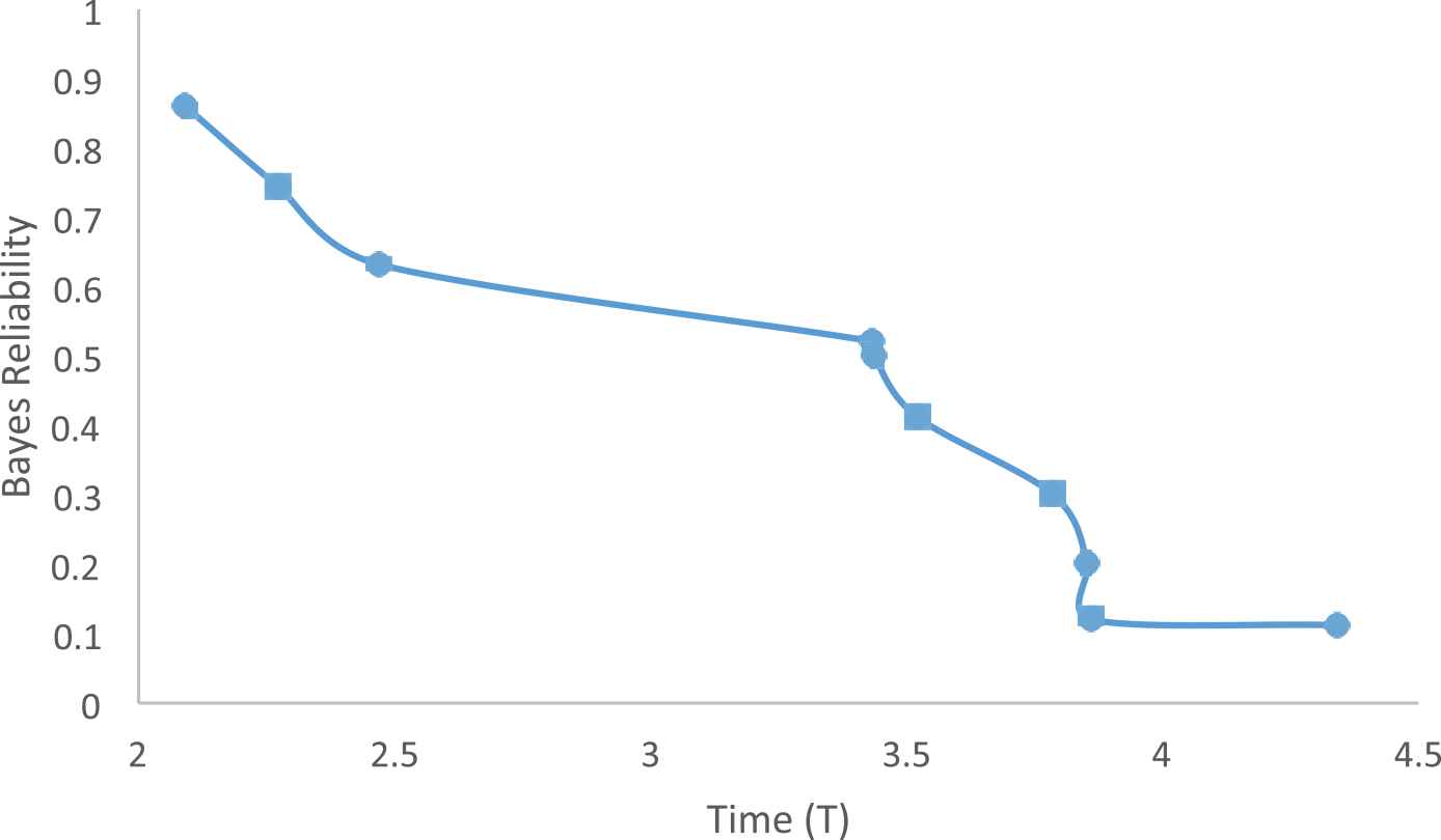
Bayes Reliability (Negative Exponential Distribution).

Minimum Unbiased Estimator (Negative Exponential Distribution).
Minimum Unbiased Estimator (Negative Exponential Distribution).
Minimum Unbiased Estimators (Weibull Distribution).
Minimum Unbiased Estimator (Weibull Distribution).
7. BAYESIAN ESTIMATION OF SYSTEM RELIABILITY WITH PRIORI RAYLEIGH DISTRIBUTION USING MONTE-CARLO SIMULATION
Consider the system consists of n s-independent two-state components. Let the time-to-failure for each component be describe by a Weibull Distribution with the pdf for i-th component failure time given by,
The shape parameter
With known parameter bi
Let one trail of the system yield the failure times, ti, for the components that fail. Let If denotes the set of the components that fail. The posterior pdf of the scale parameter of the i-th component for
Substituting the values of Equations (22) and (23) in Equation (24), we get
If
The posterior pdf can be given by
The posterior pdf of the scale parameter for these components that failed is evaluated by Equation (28) and the posterior pdf of the scale parameter for those components which does not failed is evaluated by the Equation (27).
7.1. Monte-Carlo Simulation
The posterior pdf of the scale parameter for the components can be evaluated by the above relation and can be converted to the reliability estimate for each component. We generate the values of random derivatives from the Weibull distribution. To generate
Replications of the combinations of the scale parameters generated may also be provided from the posterior pdf. Consider ks replications of scale parameter combination and kr replications of time-to-failure for each combination. The total replications are given by
If kf(t) is assumed to be the number of replications that yield system failure for required operating time t, the reliability as a function of tm is estimated by,
Now, we construct the Table 6, for generate the random derivatives by using Monte-Carlo Simulation, for different values of the parameters and we obtain the number of observations. And, we construct the Table 7, to evaluate failure time for the one trail with different parameters. In Table 8, we calculate the reliability using 200 replications for scale parameter combinations and 200 replications for time to failure given each combination, and then we estimate the reliability as the function of time. Next, we calculate the reliability using 100 replication for time to failure given each combination, and then we estimate the reliability as the function of time.
| a = c = 0.5 |
a = c = 0.8 |
||||||||
|---|---|---|---|---|---|---|---|---|---|
| Component No (i) | Random Deviations | Observations |
Shape Parameter |
Rayleigh-Priori Parameter |
Observations |
Shape Parameter |
Rayleigh-Priori Parameter |
||
| 1 | 0.123 | 2.223 | 1.0 | 2.0 | 2.033 | 3.0 | 1.0 | ||
| 2 | 0.651 | 0.091 | 1.5 | 2.2 | 0.276 | 3.5 | 1.2 | ||
| 3 | 0.868 | 0.009 | 2.0 | 2.4 | 0.068 | 4.0 | 1.4 | ||
| 4 | 0.729 | 0.049 | 2.5 | 2.6 | 0.188 | 4.5 | 1.6 | ||
| 5 | 0.798 | 0.025 | 3.0 | 2.8 | 0.123 | 5.0 | 1.8 | ||
| 6 | 0.073 | 3.400 | 3.5 | 3.0 | 2.650 | 5.5 | 2.0 | ||
| 7 | 0.490 | 0.253 | 4.0 | 3.2 | 0.523 | 6.0 | 2.2 | ||
| 8 | 0.454 | 0.310 | 4.5 | 3.4 | 0.593 | 6.5 | 2.4 | ||
| 9 | 0.107 | 2.493 | 5.0 | 3.6 | 2.183 | 7.0 | 2.6 |
Random number deviations for different values of parameters.
| Component No (i) | Time ti | Failure Time fi | Time ti | Failure Time fi |
|---|---|---|---|---|
| 1 | 0.8 | Did not fail | 0.1 | Did not fail |
| 2 | 0.9 | 0.2026 | 0.1 | 0.5772 |
| 3 | 1.0 | 0.0265 | 0.2 | 0.1799 |
| 4 | 1.2 | 0.2048 | 0.3 | 0.6562 |
| 5 | 1.3 | 0.1469 | 0.4 | 0.7487 |
| 6 | 1.4 | Did not fail | 0.5 | Did not fail |
| 7 | 1.5 | Did not fail | 0.6 | Did not fail |
| 8 | 1.6 | 0.0005 | 0.7 | 0.0022 |
| 9 | 1.7 | 0.0872 | 0.8 | Did not fail |
Results of one trail for failure time and posterior densities.
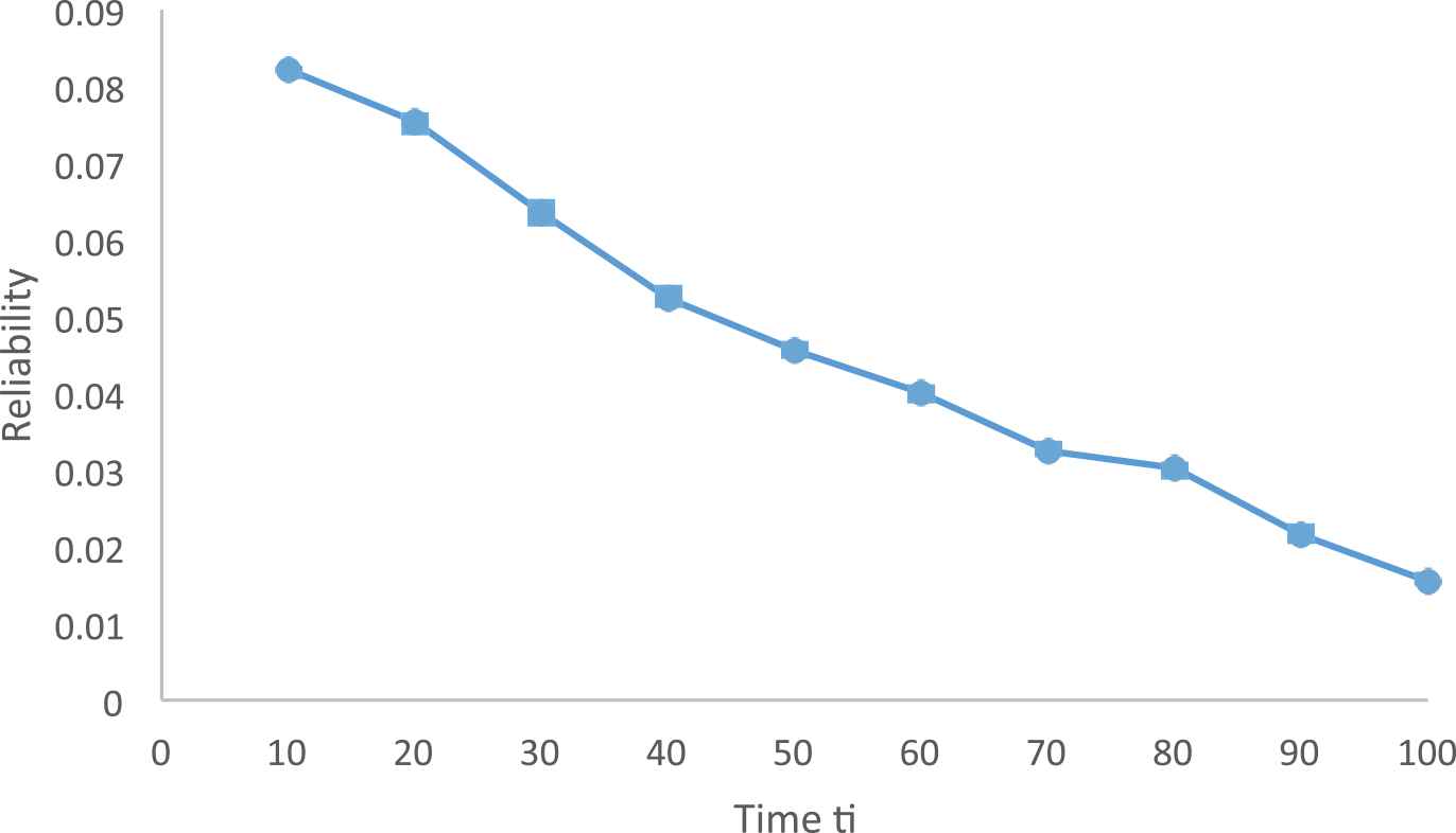
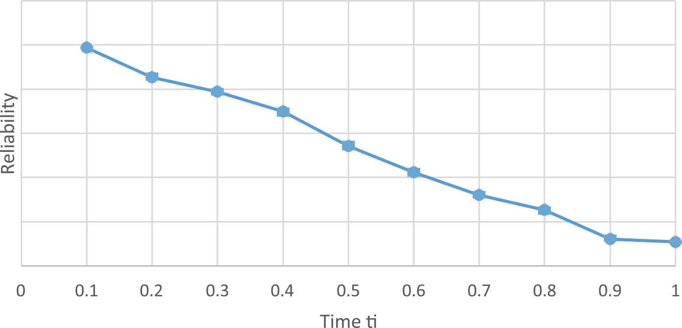
| Time ti | Reliability | Time ti | Reliability | |
|---|---|---|---|---|
| 10 | 0.0821 | 0.1 | 0.0987 | |
| 20 | 0.0754 | 0.2 | 0.0854 | |
| 30 | 0.0635 | 0.3 | 0.0789 | |
| 40 | 0.0524 | 0.4 | 0.0698 | |
| 50 | 0.0456 | 0.5 | 0.0542 | |
| 60 | 0.0400 | 0.6 | 0.0423 | |
| 70 | 0.0325 | 0.7 | 0.0321 | |
| 80 | 0.0302 | 0.8 | 0.0254 | |
| 90 | 0.0215 | 0.9 | 0.0121 | |
| 100 | 0.0155 | 1.0 | 0.0109 | |
Reliability estimation by simulation result.
And next, we illustrate the curve to demonstrate the fluctuations between the values, which help the system designers to intend the more consistent and proficient systems.
7.2. Conclusions
From Figures 7 and 8, we see that as the time increases the reliability decreases. Monte-Carlo simulation and Bayesian estimation can be combined together to estimate system reliability given systems with s-independent two-state components whose failure times are Weibull with known space parameters and Rayleigh priors for the scale parameters. With the modification can be extended to systems where shape parameters also have some priori distribution.
Reliability Estimation.
Reliability Estimation.
7.3. Necessity and Significance of the Study
The Bayesian approach is used whenever the available data for the study is too small and complex. Therefore, to resolve the objectives of the study, Bayesian estimation was used. In our study, Bayesian estimation approach is very well known and used in passenger carrying vehicle system.
In order to optimize failure rate of the vehicles, it is necessary to know the distribution of several variables. This model help to minimize the maintenance and failure rate of the passenger carrying system wherever the vehicles are in operation and standby mode.
CONFLICTS OF INTEREST
The authors declare that they have no conflicts of interest.
AUTHORS' CONTRIBUTIONS
Author 1 and 2 conceived of the presented idea, developed the models, and performed the analytic calculations and numerical simulations. Author 3 wrote the manuscript with support of Author 1. All authors discussed the results and contributed to the final manuscript.
REFERENCES
Cite this article
TY  - JOUR
AU  - Kirti Arekar
AU  - Rinku Jain
AU  - Surender Kumar
PY  - 2021
DA  - 2021/02/08
TI  - Bayesian Estimation of System Reliability Models Using Monte-Carlo Technique of Simulation
JO  - Journal of Statistical Theory and Applications
SP  - 149
EP  - 163
VL  - 20
IS  - 1
SN  - 2214-1766
UR  - https://doi.org/10.2991/jsta.d.210201.001
DO  - 10.2991/jsta.d.210201.001
ID  - Arekar2021
ER  -