
A Tutorial on Levels of Granularity: From Histograms to Clusters to Predictive Distributions
- DOI
- 10.2991/jsta.2018.17.2.10How to use a DOI?
- Keywords
- Cluster Analysis; Finite Mixture Model; Bayesian models; Compound models; prior distribution; infinite mixture
- Abstract
Consider the problem of modeling datasets such as numbers of accidents in a population of insured persons, or incidences of an illness in a population. Various levels of detail or granularity may be considered in describing the parent population. The levels used in fitting data and hence in describing the population may vary from a single distribution, possibly with extreme values, to a bimodal distribution, to a mixture of two or more distributions via the Finite Mixture Model, to modeling the population at the individual level via a compound model, which may be viewed as an infinite mixture model. Given a dataset, it is shown how to evaluate the fits of the various models by information criteria. Two datasets are considered in detail, one discrete, the other, continuous.
- Copyright
- Copyright © 2018, the Authors. Published by Atlantis Press.
- Open Access
- This is an open access article under the CC BY-NC license (http://creativecommons.org/licences/by-nc/4.0/).
1 Introduction
1.1 Background and Summary
Consider the problem of modeling a dataset of numbers accidents in a population of insured persons, or the incidence of an illness in a population. One can consider a spectrum of levels of granularity in describing the data and the corresponding population, from histograms, to a single distribution from a parametric family, to a bimodal distribution, to a mixture of two or more distributions, to modeling the population at the individual level via compound (predictive) distributions. Examples included are a dataset of employee days ill (a discrete variable) and a dataset of family expenditures on groceries (a continuous variable). Fits to the data obtained by various levels of granularity are compared using the Bayesian Information Criterion.
1.2 Levels of “Granularity”
In discussing the level at which to analyze a dataset, it will be shown how to go from individuals to histograms and modes to clusters or mixture components, back to individuals. The various levels proceed from histograms to clusters to predictive distributions
That is, one can go from modes to sub-populations back to individuals. These choices might be called choosing the level of “granularity” at which to analyze the dataset. Methods for various levels of granularity include those indicated in the table.
| Method | parameters | Model |
|---|---|---|
| Histograms | different bin widths | Multinomial |
| Cluster Analysis | parameter values for clusters of individuals | Finite Mixture Model |
| Predictive distribution | parameter value for each individual | Bayesian prior distribution |
Methods for various levels of granularity
There will be two extended analyses of datasets. These datasets are neither new nor large nor high-dimensional but hopefully will still be found to be interesting, particularly from the point of view of this paper. These two datasets are:
- •
Expenditure in a week on fruits and vegetables for 60 English families (Connor & Morrell, Statistics in Theory & Practice)
- •
Days ill in a year for 50 miners (hypothetical data from Kenkel, Statistics for Management & Economics)
2 Days Ill dataset
The first, with discrete data, concerns a (hypothetical) dataset of days ill in a year of n = 50 miners (Kenkel 1984). The days ill are of course integer values. They range from 0 to 18 days in the year.
| days | 0 | 1 | 2 | 3 | 4 | 5 | 6 | 7 | 8 | 9 | 10 | 11 | 12 | 13 | 14 | 15 | 16 | 17 | 18 |
| freq | 2 | 3 | 5 | 5 | 2 | 5 | 5 | 4 | 6 | 3 | 0 | 1 | 4 | 1 | 2 | 0 | 0 | 1 | 1 |
Frequencies of days ill
The histogram (shown here with bins 0, 1-2, 3-4, … ,17-18) suggests bimodality, with modes at about 7 days and 12 days. (Strictly speaking, it can be argued that there is an error in this figure; namely, the rectangular bar for the value 0 has the same width as that for 1-2, 3-4, etc., even though these span two values instead of one. As will be discussed below, the width should be chosen so that relative frequency is proportional to area, and area = width × height, so that the height should be doubled if the bin width is halved. This will be discussed further below.)
The sample mean is about
2.1 Extreme values
But, if one does fit a Poisson to the dataset, omitting, say, the upper two values 17 and 18 days, what conclusions might be drawn? Would the 17 and 18 be considered to be particularly unusual? That is to say, later, having fit a distribution, we can assess the probability of such extreme observations.
For now, we note that the mean of the other 50-2 = 48 observations is 5.1 days; the variance, 17.47, still very different values, so a single Poisson would not provide a good fit even after omitting the two largest, possibly outlying, observations. Note that also, besides the gap at 15 and 16 days, there is a gap at 10 days, nobody having been ill that number of days. Perhaps a mixture of distributions would make more sense.
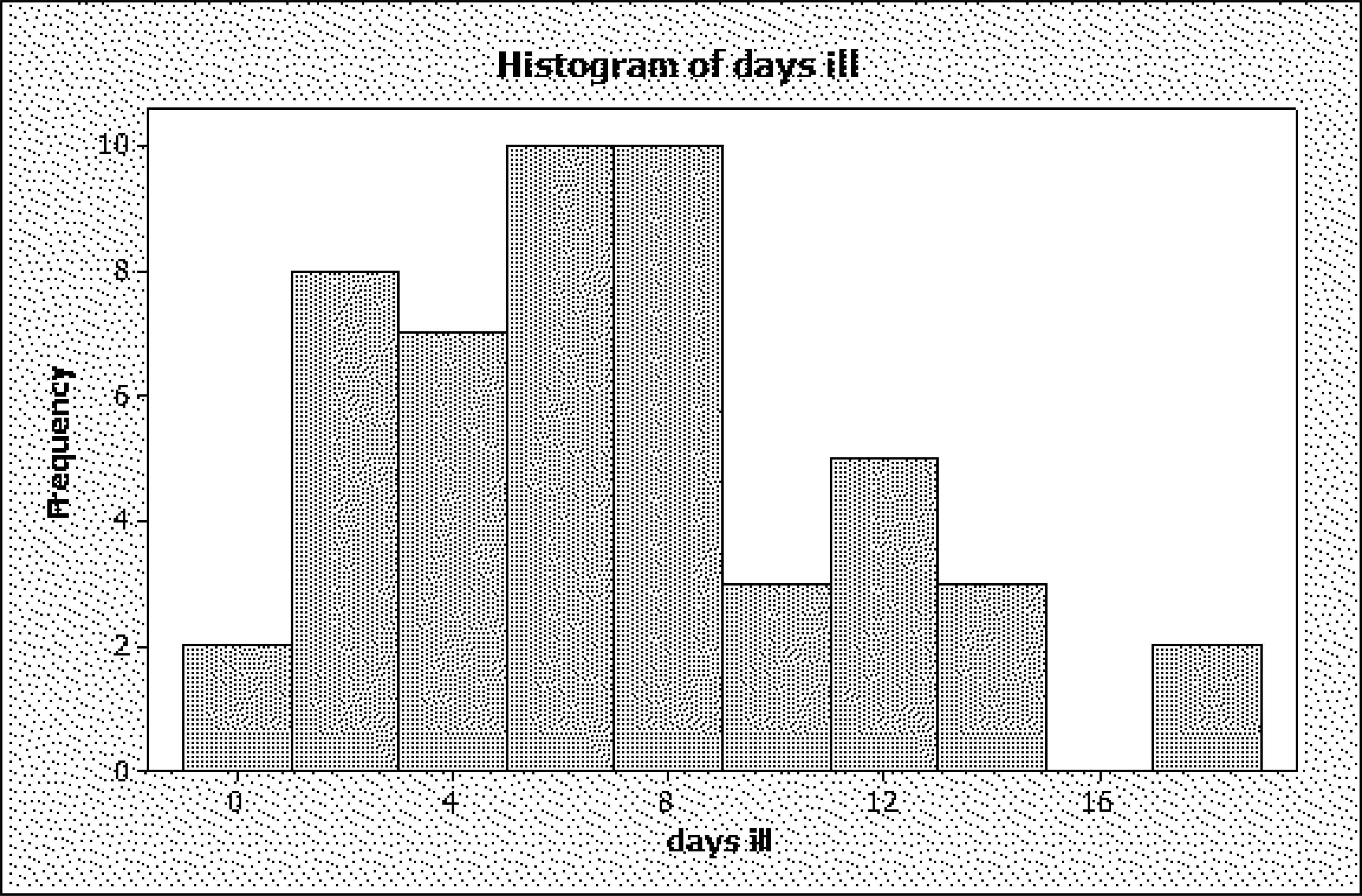
Histogram of days ill
2.2 Poisson mixture model
Consequently, a mixture of two Poissons was fit. The mixture model has p.m.f. (probability mass function) p(x) = π1 p1(x) + π2 p2(x), where p1(·) is the p.m.f. of a Poisson distribution with parameter λ1 and p2(·) is the p.m.f. of a Poisson distribution with parameter λ2.
Parameter estimates for the Poisson mixture model. Starting values for iterative estimation were obtained by a Student’s t method of clustering into two groups (Sclove 2016). In this method, each cut-point is tried.
In more detail: Obtain the order statistic, resulting from ordering the the observations {x1, x2, … , xn} as
Candidate cut-off points c1, c2, … , cn−1 are chosen in between the order statistics:
For example, one can take cj to be the midpoint cj = (x(j) + x(j + 1))/2. One then computes two-sample t for each clustering, that is, for each cut-point. The best clustering into two clusters is the one which gives the largest value of |t|, or, equivalently, of t2. This is because t2 compares the within-groups sum of squares and the between-groups sum of squares.
Pooled t assumes equal variances in the two clusters. Unpooled t avoids this assumption. Not assuming equal variances, one can consider the standardized difference between means as an objective function, that is, one can use an unpooled two-sample t as the criterion, maximizing it over cut points. The unpooled t statistic is given by
The value of the two-sample, unequal variance Student’s t is computed for each cut-point, and the cut-point giving the largest t2 is chosen.
Iteration. The means of the resulting clusters are taken as tentative estimates of the distributional means; the cluster relative frequencies, as tentative estimates of the mixing probabilities. These estimates were 2.1 days, 8.9 days, with cluster frequencies of 17 out of 50 and 33 out of 50, that is, mixing probabilities of .34, .66. By doing a grid search in the vicinity of these initial estimates to maximize the mixture-model likelihood, the following estimates were obtained:
Extreme value assessment with the fitted Poisson mixture. With the fitted Poisson mixture, the estimate of Pr{X > 16} is .007, fairly small. So perhaps results of 17 or more days could and should be considered outliers.
2.3 Comparison of models by model-selection criteria
The two fits, by histogram and by Poisson mixture, were compared by means of model-selection criteria. Given K alternative models, indexed by k = 1, 2, … , K, penalized-likelihood model-selection criteria are smaller-is-better criteria that can be written in the form
The number of parameters for the Poisson mixture is 2 means plus 2 mixing probabilities, less 1 because the probabilities must add to 1. That is 3 free parameters for the Poisson mixture. The number of parameters for the histogram, scored by the multinomial distribution with 17 categories (0 through 18, but 15 and 16 are missing), less 1 because the multinomial probabilities must add to 1, leaving 16 free parameters.
The results are in the next table. The histogram wins by a bit according to AIC, but the Poisson mixture wins by a wide margin according to BIC. To see this, note that BIC is derived (Schwarz 1978) as the first terms in the Taylor series expansion of (-2 times) the posterior probability of Model k, Pr(Model k | data) = ppk, say. That is,
| Model, k | − 2 LLk | mk | AICk | BICk | ppk |
|---|---|---|---|---|---|
| k = 1 : histogram | 261.642 | 16 | 293.642 | 324.234 | 5.0 × 10⁻⁷ |
| k = 2 : Poisson mixture | 283.473 | 3 | 289.473 | 295.209 | ≈ 1 |
Comparison of two models
| Model, k | BICk | same - 295 | exp(−same/2) | ppk |
|---|---|---|---|---|
| 1 | 324.234 | 29.234 | 4.5 × 10⁻⁷ | 4.98 × 10⁻⁷ |
| 2 | 295.209 | 0.209 | 0.90085 | 1.000 |
| sum = | 0.90085 | |||
Calculation of posterior probabilties of alternative models
To calculate the posterior probabilities, one subtracts a large constant from each, divides by 2, exponeniates the negative of this, and sums these, dividing by the sum to normalize.
Different bin widths. If one makes several histograms, with different bin widths, how should the likelihood for histograms be computed? Given data points x1, x2, … , xn, the likelihood for a given p.m.f. p(·) is
Here p(xi) is the p.m.f. at the data point xi. (For continuous data, we would write the p.d.f., f(xi). ) But in the context of histograms what we can take p(xi) to be?
Denote the number of bins by J. Let the bin width be denoted by h. This is an increment along the x-axis.
Let the bins be indexed by j, j = 1, 2, … , J. The class limits are x0, x0 + h, x0 + 2h, … , x0 + Jh. The class intervals (bins) are [x0, x0 + h), [x0 + h, x0 + 2h), … , [x0 + (J − 1)h, x0 + Jh). In the present application, x0 = 0. Now, let j(xi) denote the bin containing xi and nj(xi) be the frequency in that bin. To approximate f(xi), motivated by f(x1) ≈ [F(x2) − F(x1)]/(x2 − x1) = [F(x1 + h) − F(x1)]/[(xi + h) − x1] = [F(x1 + h) − F(x1)]/h, write
That is, the concept is that probability density is probability per unit length along the x axis. Thus the likelihood is
Note that
Varying bin widths. In the case of non-constant bin widths, with a bin-width of hj for the j-th interval, take the probability density at xi to be nj(i)/hj(i), where hj(i) is the width of the interval in which xi falls and nj(i) (short for nj(xi) ) is the frequency (count) in that interval. The likelihood is
| days | 0 -1 | 2-3 | 4-5 | 6-7 | 8- 9 | 10- 11 | 12- 13 | 14- 15 | 16-17 | 18-19 |
| freq | 5 | 10 | 7 | 9 | 9 | 1 | 5 | 2 | 1 | 1 |
Sample distribution with a bin width of 2
| days | 0 | 1 | 2-3 | 4-5 | 6-7 | 8- 9 | 10- 11 | 12- 13 | 14- 15 | 16-17 | 18 |
| bin width | 1 | 1 | 2 | 2 | 2 | 2 | 2 | 2 | 2 | 2 | 1 |
| freq | 2 | 3 | 10 | 7 | 9 | 9 | 1 | 5 | 2 | 1 | 1 |
Sample distribution with varying bin widths: bins 0, 1, 2-3,4-5.6-7, … , 16-17, 18
According to AIC, the histogram with varying bin widths wins, the Poisson mixture coming in second. According to BIC (and, equivalentlly, posterior probability), the Poisson mixture scores the best, by far. But the point is not just which model wins, but that such a comparison, comparing histograms on the one hand with fitted distributions on the other, can be made.
Levels of granularity, cont’d. Perhaps another level of granularity is approached by predictive distributions, which may be viewed as getting to the individual level of granularity. Predictive distributions may be viewed in the light of compound distributions resulting from a prior distribution on the parameter at the individual level. From the viewpoint of modern statistics, a predictive distribution is merely the marginal distribution of the observable random variable, having integrated out the prior on the parameter. (Details to follow.)
The Yule-Greenwood model approaches modeling at the individual level, stating that each individual may have his or her own accident rate λ and so is an example of a compound model. In terms of granularity, the Yule-Greenwood model is a classical example at the level of the individual in that it employs a Poisson model for each individual’s accident rate λ and then puts a (Gamma) distribution over the population of values of λ. The model is the Gamma-Poisson model (sometimes called the Poisson-Gamma model) and is a prime example of a compound model. The Gamma is a conjugate prior distribution for the Poisson, meaning that the posterior distribution of λ is also a member of the Gamma family. We discuss this further below; first, however, we fit histograms and mixtures to a dataset with continuous data.
3 An example with continuous data
The variable in the next example is expenditure in a week (£) of n = 60 English families on fruits and vegetables (Connor and Morrell 1977, data from the British Institute of Cost and Management Accountants). The data are reported to two decimals. This sort of measurement, treated as continuous, contrasts with the integer-valued variable considered in the example above.
Here are the data, sorted from smallest to largest:
0.21, 0.33, 0.36, 0.38, 0.41, 0.46, 0.48, 0.48, 0.51, 0.51, 0.51, 0.58, 0.64, 0.66, 0.69, 0.69, 0.71, 0.74, 0.74, 0.78, 0.78, 0.79, 0.84, 0.87, 0.87, 0.88, 0.89, 0.91, 0.91, 0.93, 0.98, 0.98, 1.03, 1.03, 1.05, 1.08, 1.12, 1.16, 1.17, 1.19, 1.24, 1.25, 1.26, 1.26, 1.28, 1.33, 1.38, 1.44, 1.48, 1.51, 1.53, 1.58, 1.61, 1.62, 1.76, 1.78, 1.79, 1.83, 1.96, 2.13
The minimum is 0.21 £; the maximum, 2.13 £. The sample mean is
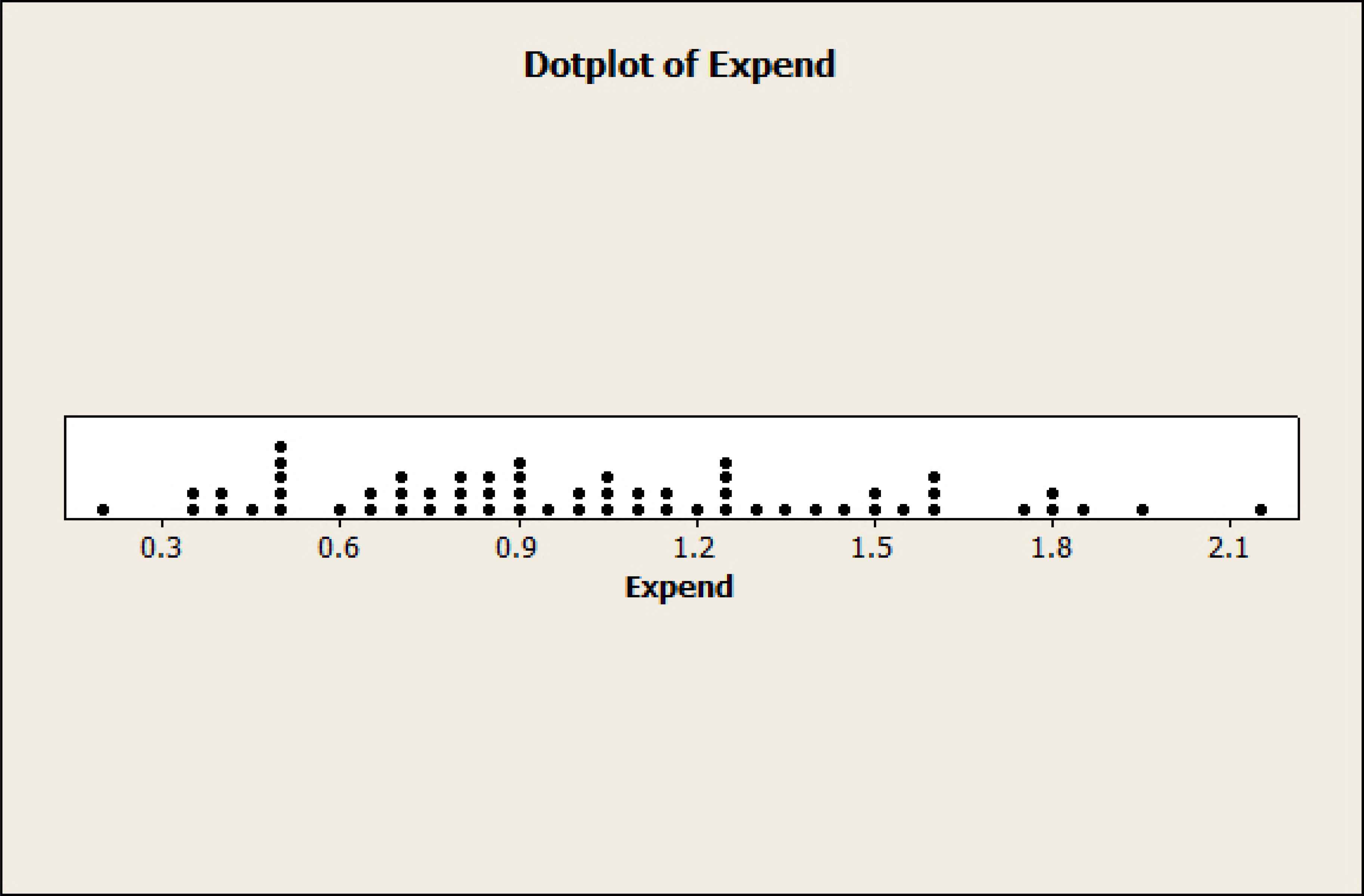
Dotplot of Expenditure
| Model, k | − 2 LLk | mk | AICk | BICk | ppk |
|---|---|---|---|---|---|
| histogram, bin width h=1 | 261.6 | 16 | 293.6 | 324.2 | .000 |
| histogram, bin width h=2 | 273.2 | 9 | 291.2 | 308.4 | .001 |
| histogram, varying bin widths | 267.8 | 9 | 285.8 | 303.0 | .020 |
| Poisson mixture | 283.5 | 3 | 289.5 | 295.2 | .978 |
Comparison of models
| lower limit | 0.21 | 0.31 | 0.41 | 0.51 | 0.61 | 0.71 | 0.81 | 0.91 | 1.01 | 1.11 |
| upper limit | 0.30 | 0.40 | 0.50 | 0.60 | 0.70 | 0.80 | 0.90 | 1.00 | 1.10 | 1.20 |
| Frequency | 1 | 3 | 4 | 4 | 4 | 6 | 5 | 5 | 4 | 4 |
| lower limit | 1.21 | 1.31 | 1.41 | 1.51 | 1.61 | 1.71 | 1.81 | 1.91 | 2.01 | 2.11 |
| upper limit | 1.30 | 1.40 | 1.50 | 1.60 | 1.70 | 1.80 | 1.90 | 2.00 | 2.10 | 2.20 |
| Frequency | 5 | 2 | 2 | 3 | 2 | 3 | 1 | 1 | 0 | 1 |
Frequency distribution of weekly expenditure (£)
The distribution as tabulated here has a bin width h of 0.10. We consider below also the results for h = 0.2, for fitting a single Gamma and also for fitting a mixture of two (Gaussian) distributions. Below we compare these four fits by means of AIC and BIC.
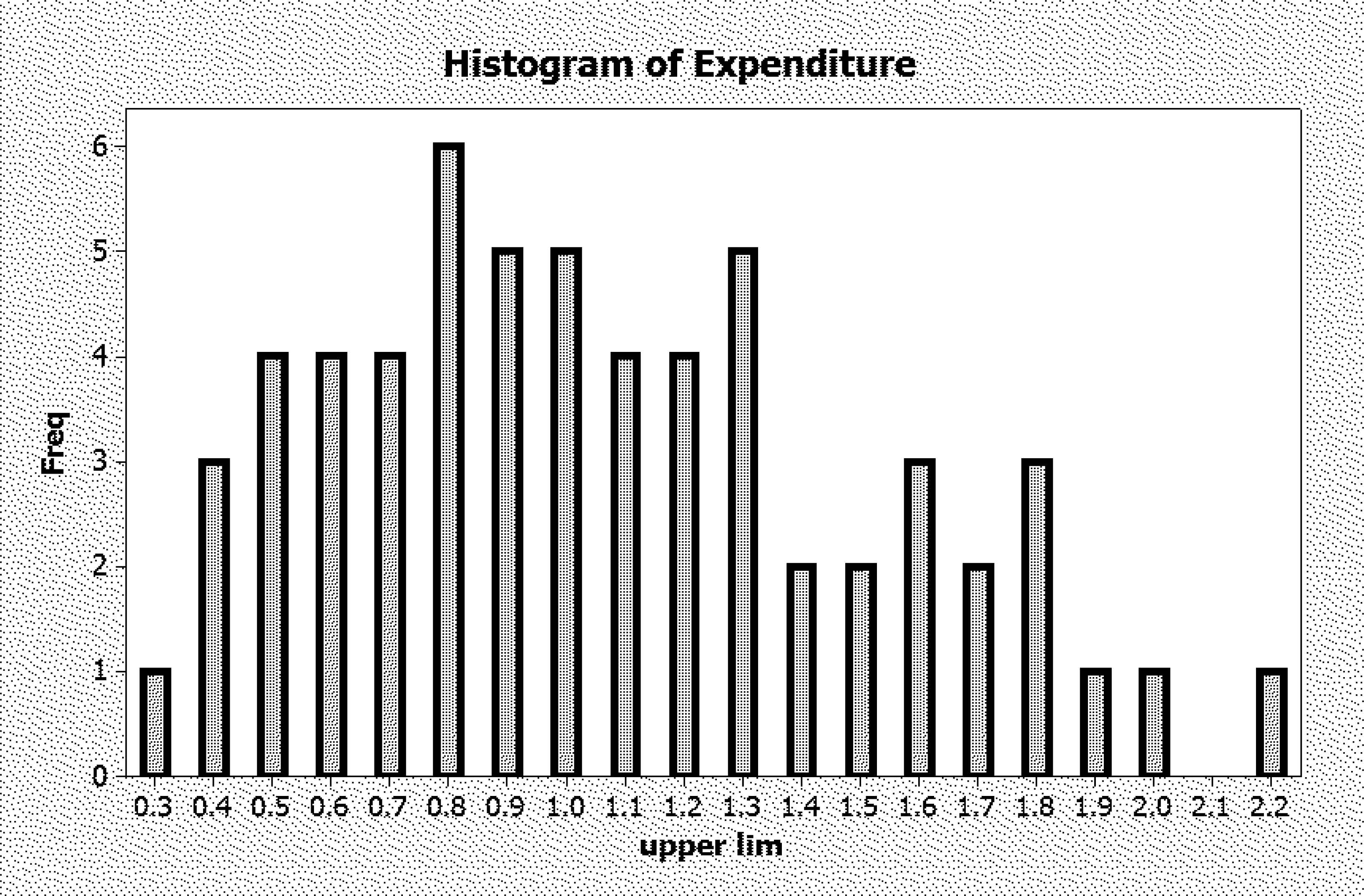
Histogram of Expenditure
3.1 Fitting a Gamma distribution
The two-parameter Gamma p.d.f. is
The mean is mβ. The variance is mβ2. Method-of-moments estimates are, for the scale parameter β = σ2/μ,
3.2 Fitting mixture models
3.2.1 Gaussian mixture
The mixture model has p.d.f. f(x) = π1 f1(x) + π2 f2(x), where f1(·) is the p.d.f. of a Gaussian distribution with mean μ1 and variance
Then the estimates are updated. (See McLachlan and Peel (2000), p. 82.) For j = 1, 2,
As a check, note that if for one group j, it happened that pp(s)(j|xi) = 1 for all cases i, then the new estimate of the mean for that j is simply
Then, variance equals raw second moment minus square of mean, or
Note that the numerical estimates of σ1 and σ2 are somewhat different; the ratio of variances is (0.27/0.23)2 = 0.075/0.051 = 1.46. Given this, it does not seem particularly worthwhile in this case to trying fitting two Gaussians with equal variances.
The table summarizes the results. According to AIC, the ranking is: Gamma, Gaussian mixture; histogram with bin width .2, histogram with bin width .1. According to BIC, the ranking is: Gaussian mixture, Gamma, histogram with bin width .2, histogram with bin width .1.
| Model, k | − 2 LLk | mk | AICk | BICk | ppk |
|---|---|---|---|---|---|
| histogram, bin width h=0.1 | 61.68 | 18 | 97.68 | 135.38 | .000 |
| histogram, bin width h=0.2 | 66.25 | 9 | 84.25 | 103.10 | .000 |
| Gamma | 71.75 | 2 | 75.75 | 79.94 | .382 |
| Gaussian mixture | 70.79 | 5 | 80.79 | 78.98 | .618 |
Comparison of results
3.2.2 Gamma mixture
The mixture model has p.d.f. f(x) = π1 f1(x) + π2 f2(x), where now f1(·) is the p.d.f. of a Gamma distribution with shape parameter m1 and scale parameter β1 and f2(·) is the p.d.f. of a Gamma distribution with shape parameter m2 and scale parameter β2. The means and variances are, for distributions j = 1, 2, μj = mjβj and
The resulting estimates are
The results were obtained by approximate maximization of the likelihood doing an EM (Expectation-Maximization) iteration. Starting values were obtained by the Student’s t method (Sclove 2016).
Given starting values μ1(0),
Then the estimates are updated. For j = 1, 2,
As a check, note that if for one group j, it happened that pp(s)(j|xi) = 1 for all cases i, then the new estimate of the mean for that j is simply
Then, of course, variance equals raw second moment minus square of mean, or
Then these are converted to updated estimates of mj, βj, and the iteration continues until satisfactory convergence. LL, AIC, and BIC are computed with the resulting estimates.
3.3 Comparison of models by model-selection criteria
The table summarizes the results. According to AIC, the ranking is: Gamma; Gaussian mixture; Gamma mixture; histogram with bin width .2, histogram with bin width .1. According to BIC, the ranking is: Gaussian mixture, Gamma, Gamma mixture, histogram with bin width .2, histogram with bin width .1 The Gamma mixture has only a small posterior probability.
| Model, k | − 2 LLk | mk | AICk | BICk | ppk |
|---|---|---|---|---|---|
| histogram, bin width h=0.1 | 61.68 | 18 | 97.68 | 135.38 | .000 |
| histogram, bin width h=0.2 | 66.25 | 9 | 84.25 | 103.10 | .000 |
| Gamma | 71.75 | 2 | 75.75 | 79.94 | .382 |
| Gaussian mixture | 70.79 | 5 | 80.79 | 78.98 | .617 |
| Gamma mixture | 71.75 | 5 | 81.75 | 92.22 | .001 |
Comparison of results
4 Compound Models in General
First, notation notation for probability functions will be reviewed.
The probability density function (p.d.f.) of a continuous random variable (r.v.) X, evaluated at x, will be denoted by fX(x). The p.d.f. of a continuous random variable Y, evaluated at y, is similarly denoted by fY(y).
Now consider a bivariate variable x = (y, z). The joint p.d.f. of the r.v.s Y and Z, evaluated at (y, z) is fY,Z(y, z). Example: Y = WT, X = HT, the value of the joint p.d.f. at y = 80 kg and z = 170 cm is fWT,HT (80, 170).
Other notations include:
fY|X(y|x): conditional probability density function of the r.v. Y, given that the value of the r.v. X is x. Example: fWT|HT(wt | HT = 170cm). This represents the bell-shaped curve of weights for men of height 170 cm.
fY,Z(y | z) = fY|Z(y|z) fZ(z): This is the joint p.d.f. expressed as the product of the conditional of Y given Z and the marginal of Z
fY(y) = ∫ fY,Z(y, z) dz = ∫ fY|Z(y|z) fZ(z) dz: marginal p.d.f. of Y
In the development that follows, fZ(z) plays the role of the prior probability function on the parameter. That is, denoting the parameter by θ, the function fZ(z) will become fΘ(θ).
The elements of compound models are:
- •
The distribution of the observable r.v., given the parameter(s), that is, the conditional distribution of X, given the parameter(s); and the marginal distribution (predictive distribution). The marginal distribution will have the hyperparameters among its parameters.
- •
the prior distribution. Its parameters are called hyperparameters.
A generic symbol for the parameter(s) of the conditional distribution of X is the conventional θ. As a generic symbol for the hyperparameters, one could use α, since the prior comes first in the model when one thinks of the parameter value being given first, and then the value of the variable being observed.
For use in compound models, the probability functions include the following:
The conditional distribution of the observable r.v. X, given the value of the parameter, is fX|Θ(x|θ); p.d.f. of X for given θ.
The prior distribution on the parameter θ with hyperparameter vector α, fΘ(θ; α).
The naming of compound models takes the form, prior distribution – conditional distribution. In the Gamma-Poisson model, the conditional distribution of X given λ is Poisson(λ) and the prior distribution on λ is Gamma. In the Beta-Binomial mode, the conditional distribution of X given p is Binomial with success probability p and the prior distribution on p is Beta. (Note that some people use the form, conditional distribution – prior distribution, e.g., Poisson-Gamma.)
5 The Gamma-Poisson model
5.1 Probability functions for the Gamma-Poisson model
In the Gamma-Poisson model, the distribution of X is Poisson with parameter usually called λ. The p.m.f. is
The mean and variance are both equal to λ.
Such a distribution can be considered, say, for the number of accidents per individual per year. For the days ill dataset (days ill in a year for a sample of n = 50 miners), we have fit a single Poisson (with mean 6.58 days per year). We looked at histograms and observed bimodality. Further, the fact that the sample variance of 19.06 was considerably larger than the sample mean was a hint of inadequacy of a single Poisson. As discussed above, a mixture of Poissons was fitted, with mixing probabilities about .6 and .4 and means about 3 days and 9 days. A finer level of granularity would be obtained by saying that each person has his own value of λ and putting a distributon on these over the population.
5.2 Gamma family of distributions
A Gamma distribution could be a good choice. The choice of the Gamma family is non-restrictive in that the family can achieve a wide variety of shapes. The single-parameter gamma has a shape parameter m; the two-parameter gamma family has, in addition, a scale parameter, β. (The reciprocal of β is the rate parameter, so-called because it is the rate, or intensity, of the associated Poisson process.) A Gamma distribution with parameter m, has p.d.f. f(λ) = Const. λm−1 e−λ, λ > 0. The constant is 1/Γ(m). More generally, the two-parameter Gamma can be used: the p.d.f. is
The mean is mβ. The variance is mβ2.
The Negative Exponential family of distributions. The special case of m = 1 in the Gamma family gives the negative exponential family of distributions. So the
The mean is β. The variance is β2.
5.3 Development of the Gamma-Poisson model
Putting a population distribution over a parameter can be a very helpful way of modeling. The resulting model is called a compound model. In a compound model, the random variable X is considered as the result of sampling that yields an individual and that individual’s value of a parameter, and then the individual’s value of X is observed, from a distribution with that value of the parameter. Note that a compound model can be viewed as an infinite mixture model.
In this discussion, focus is on a couple of particular compound models, the Gamma-Poisson, and later, the Beta-Binomial.
The Yule-Greenwood model, from a modern viewpoint, is an application of the Gamma-Poisson model to a financial, in fact, actuarial, situation. It is in terms of a model for accident rates in a population. Suppose that the yearly number of accidents of any given individual i in a population is distributed according to a Poisson distribution with parameter λi accidents per year. (This is count data, similar to the days ill data.) Then the probability that individual i, with parameter value λi, has exactly k accidents in a year, k = 0, 1, 2, … , is
Some individuals are more accident prone (have a higher accident rate) than others, so different individuals have different values of λ. A distribution can be put on λ to deal with this. This is the Yule-Greenwood model, dating from 1920; a precursor of the Predictive Distributions of the new Predictive Analytics, predating even Abraham Wald (1950) as a founder of modern mathematical statistics and decision theory and Jimmie Savage (1954) as a founder of modern Bayesian Statistics.
The standard choice of a prior distribution on λ is a Gamma distribution. The Gamma family is a conjugate family to the Poisson, meaning that the prior and posterior distributions of λ are both in the Gamma family.
The joint distribution of X and Λ. The joint probability function of X and Λ is
The expressions for the Gamma and Poisson are put into this. That is, the weight assigned to pX||Λ(x|λ) is fΛ(λ).
The joint probability function is used to obtain
- •
the marginal distribution of X, by integrating out λ, and
- •
then the posterior distribution of Λ given x, by dividing the joint probability function by the marginal probability mass function of X.
Putting in the expressions for the Gamma and Poisson, it is seen that the marginal distribution of X, the number of accidents that a randomly selected individual has in a year, is of the form
When the prior is Gamma and the conditional is Poisson, this marginal distribution can be shown to be negative binomial. Its parameters are m and p = 1/(1 + β).
In the Bayesian model, the parameter of the conditional distribution of X, say θ, is treated as a random variable Θ.
In the Gamma-Poisson model, θ is the Poisson parameter λ.
The conditional distribution of X given that Θ = θ is Poisson(λ). The probability mass function is
The joint p.d.f. of X and Λ can be written as pX||Λ(x|λ) which is fΛ(λ)(x, λ) = fΛ pX|Λ(x|λ.
As mentioned above, from this, the posterior distribution of Λ, that is, the distribution of Λ given x, can be computed, and the marginal distribution of X can be computed. Marginal maximum likelihood estimation can be applied to obtain estimates of the remaining parameters.
Posterior distribution of Λ. Analogous to Pr(B|A) = Pr(A ∩ B) / Pr(A), the p.d.f. of the posterior distribution is the joint p.d.f., divided by the marginal p.d.f. of X :
This will turn out to be a Gamma distribution, that is, it is in the same family as the prior. The Gamma is a conjugate prior for the Poisson.
Marginal distribution of X. In Predictive Analytics, the marginal distribution of X is computed as a model of a future observation or observations of X.
The marginal distribution of X is obtained by integrating the joint distribution with respect to the parameter. Note that this computation combines information, by weighting the conditional distribution of X given λ with the prior on λ. This computation of the p.d.f. is, as stated above,
Moments. The mean of the marginal distribution of X is mq/p = m β. The variance of the marginal distribution of X is mq/p2 = m β(1 + β).
5.4 Empirical Bayes estimation
Empirical Bayes estimation, at least in the present context, means estimating the parameters of the prior using observations from the marginal distribution.
The hyperparameters in terms of the moments of the marginal. The parameters of the prior are called hyperparameters. In this case, they are λ and β. Suppose we solve for them in terms of the first two moments of the marginal.
Estimating the prior parameters from the marginal. Estimates of the prior parameters m and β can be obtained by, for example, taking the expressions for the hyperparameters m and β in terms of the first two raw moments and plugging in estimates
5.5 Application to the days ill dataset
Returning to the days ill dataset for n = 50 miners, the days ill in a year ranged from 0 to 18; the distribution seems to be bimodal.
The p.m.f. of the Negative Binomial distribution with parameters m and p is where k is the number of trials in excess of m required to get m Heads. In the Gamma-Poisson model, the marginal distribution of X is Negative Binomial with parameters with parameters m and p = 1/(1 + β).
Given that the true mean of the marginal (“predictive distribution”) Negative Binomial is μ = mq/p = mβ and the true variance is σ2 = mq/p2 = mβ(1 + β), and the sample mean
The equations are [1] : m β = 6.58; [2] : m β(1 + β) = 19.07.
Putting [1] in [2] gives 6.58(1 + β) = 19.07, 1 + β = 19.07/6.58 ≈ 2.898,
To estimate the mean and variance of the Gamma prior, one can proceed as follows. The mean of the prior is mβ, estimated as 6.58 days ill per year. The variance of the prior is mβ2, estimated as 6.58(1.898) ≈ 12.49. The standard deviation is thus estimated as
Maximum likelihood estimates are not in closed form but numerical values for them could be obtained by numerical maximization of the likelihood function. It is helpful to use the method of moments as a quick and simple method to get an idea of the values of the parameters.
The table includes the marginal negative binomial with m = 3 and p = .344 in the comparison.
| Model, k | − 2 LLk | mk | AICk | BICk | ppk |
|---|---|---|---|---|---|
| histogram, bin width h=1 | 261.6 | 16 | 293.6 | 324.2 | .000 |
| histogram, bin width h=2 | 273.2 | 9 | 291.2 | 308.4 | .000 |
| histogram, varying bin widths | 267.8 | 9 | 285.8 | 303.0 | .002 |
| Poisson mixture | 283.5 | 3 | 289.5 | 295.2 | .100 |
| marginal Negative Binomial | 283.0 | 2 | 286.0 | 290.8 | .898 |
Comparison of models, cont’d
According to AIC, the histogram with varying bin widths still wins, the Negative Binomial coming in second. According to BIC (and, equivalentlly, posterior probability), the Negative Binomial scores the best, by far. This Negative Binomial is unimodal with a mode of .115 at 3 days. Because it is unimodal, it perhaps does not capture the flavor of the original data, which is reflected better by the Poisson mixture.
6 Some other compound models: Beta-Binomial; Normal-Normal
6.1 Beta-Binomial model
Another compound model is the Beta-Binomial model.In this model, the conditional distribution of X given p is Binomial(n,p). The prior on p is Beta(α, β). The posterior distribution of p given x is Beta(α + x, β + n − x). It is as if there had been a first round of α + β trials, with α successes, followed by a second round of n trials, with x successes. Method of Moments estimates of the parameters of the prior can be relatively easilty obtained. So can the Bayes estimates.
6.2 Normal-Normal model
We have considered the Gamma-Poisson model and, briefly, another prominent compound model, the Beta-Binomial model, with a Beta prior on the Binomial success probability parameters. Still another compound model is the Normal-Normal model.
In the Normal-Normal model, X is distributed according to 𝒩(μ, σ2), the Gaussian distribution with mean μ and variance σ2. The prior on μ can be taken to be
The posterior distribution is again Normal. That is, the Normal family is the conjugate family for the Normal distribution. The marginal distribution is also Normal, with mean ℰ[X] = ℰ[ℰ[X|μ] = ℰ[μ] = μ0. The variance of the marginal distribution is the mean of the conditional variance plus the variance of the conditional mean,
7 Proposed Extensions and Issues
Multivariate models. Multivariate generalizations, where the response is a vector rather than a scalar, could be interesting, both in general and in the context of the analysis of variance.
Parameter-space boundary issues. Chen and Szroeter (2016) provide a more widely applicable version of BIC (originally called the Schwarz Information Criterion, SIC). This version deals with boundary issues in the parameter space. These issues can be important when dealing with mixture models, as the parameter space changes as the number of component distributions changes..
A BIC for Maximum Marginal Likelihood. In view of the fact that, in this paper, compound models have been mentioned as a level of granularity for modeling at the individual level, it is worth mentioning that Spiegelhalter et al. (2002) use an information theoretic argument to derive a measure pD for the effective number of parameters in a model as the difference between the posterior mean of the deviance and the deviance at the posterior means of the parameters of interest. In general this measure pD approximately corresponds to the trace of the product of Fisher’s information and the posterior covariance, which in normal models is the trace of the ’hat’ matrix projecting observations onto fitted values, that is, the matrix of estimated regression coefficients. The properties of the measure in exponential families are explored in their paper. The posterior mean deviance is suggested as a Bayesian measure of fit or adequacy, and the contributions of individual observations to the fit and complexity can give rise to a diagnostic plot of deviance residuals against leverages. Adding pD to the posterior mean deviance gives a deviance information criterion for comparing models, which is related to other information criteria and has an approximate decision theoretic justification.
Acknowledgments
An earlier version of this paper was presented at the 2016 Annual Meeting of the Classification Society, June 1-4, 2016, University of Missouri, and also at ICOSDA 2016, the 2016 International Conference on Statistical Distributions and Applications, October 14-16, 2016, Niagara Falls, Ontario, Canada, organized by Professor Ejaz Ahmed of Brock University and Professors Felix Famoye and Carl Lee of Central Michigan University. This paper was presented in the topic-invited session ”Extreme Value Distributions and Models”, organized by Professor Mei Luang Huang, Brock University; sincere thanks are extended to Professor Huang for the invitation to speak at the conference.
Bibliography.
The books mentioned below on predictive analytics, those of Murphy and Bishop, do not discuss the Gamma-Poisson model explicitly. Those who wish to consult these books may however refer to them to find Murphy, p. 41 on the Gamma family of dsitributions and/or Bishop, p. 688 on the Gamma family. As mentioned, an original paper, anticipating the subject of compound models, is that of Major Greenwood and G. Udny Yule (1920). To review background in Probability Theory in general, see, for example, Emanuel Parzen (1992) or Sheldon Ross (2014). See also Parzen, Stochastic Processes (1962) or Ross, Applied Probability Models (1970).
References
Cite this article
TY  - JOUR
AU  - STANLEY L. SCLOVE
PY  - 2018
DA  - 2018/06/30
TI  - A Tutorial on Levels of Granularity: From Histograms to Clusters to Predictive Distributions
JO  - Journal of Statistical Theory and Applications
SP  - 307
EP  - 323
VL  - 17
IS  - 2
SN  - 2214-1766
UR  - https://doi.org/10.2991/jsta.2018.17.2.10
DO  - 10.2991/jsta.2018.17.2.10
ID  - SCLOVE2018
ER  -