BAYESIAN APPROACH IN ESTIMATION OF SHAPE PARAMETER OF THE EXPONENTIATED MOMENT EXPONENTIAL DISTRIBUTION

Kawsar Fatima; S.P Ahmad*

doi:10.2991/jsta.2018.17.2.13

<Previous Article In Issue

Download article (PDF)

Next Article In Issue>

Volume 17, Issue 2, June 2018, Pages 359 - 374

BAYESIAN APPROACH IN ESTIMATION OF SHAPE PARAMETER OF THE EXPONENTIATED MOMENT EXPONENTIAL DISTRIBUTION

Authors

Kawsar Fatimakawsarfatima@gmail.com

Department of Statistics, University of Kashmir, Srinagar, India

S.P Ahmad*rosheeba2@gmail.com

Department of Statistics, University of Kashmir, Srinagar, India

Received 1 November 2016, Accepted 19 June 2017, Available Online 30 June 2018.

DOI: 10.2991/jsta.2018.17.2.13 How to use a DOI?
Keywords: Exponentiated Moment Exponential distribution; Maximum Likelihood Estimator; Bayesian estimation; Priors; Loss functions
Abstract: In this paper, Bayes estimators of the unknown shape parameter of the exponentiated moment exponential distribution (EMED)have been derived by using two informative (gamma and chi-square) priors and two non-informative (Jeffrey’s and uniform) priors under different loss functions, namely, Squared Error Loss function, Entropy loss function and precautionary Loss function. The Maximum likelihood estimator (MLE) is obtained. Also, we used two real life data sets to illustrate the result derived.
Copyright: Copyright © 2018, the Authors. Published by Atlantis Press.
Open Access: This is an open access article under the CC BY-NC license (http://creativecommons.org/licences/by-nc/4.0/).

1. Introduction

The exponentiated exponential distribution is a specific family of the exponentiated Weibull distribution. In analyzing several life time data situations, it has been observed that the dual parameter exponentiated exponential distribution can be more effectively used as compared to both dual parameters of gamma or Weibull distribution. When we consider the shape parameter of exponentiated exponential, gamma and Weibull is one, then these distributions becomes one parameter exponential distribution. Hence, these three distributions are the off shoots of the exponential distribution. Moment distributions have a vital role in mathematics and statistics, in particular probability theory, in the viewpoint research related to ecology, reliability, biomedical field, econometrics, survey sampling and in life-testing. One of such distributions is the two-parameter weighted exponential distribution introduced by [8]. [3] Proposed a distribution function of moment exponential distribution and developed some basic properties like moments, skewness, kurtosis, moment generating function and hazard function. Bayes estimators for the weighted exponential distribution (WED) was considered by [6] while [1] compare the priors for the exponentiated exponential distribution under different loss functions. [13] Obtained the Bayes estimators of length biased Nakagami distribution. [9] Proposed exponentiated moment exponential distribution (EMED) with cdf given by

(1.1)F(x)=[1−x+ββe−xβ]α, x>0,α,β>0,

where α is the shape parameter and β is the scale parameter and exponentiated moment exponential distribution and is denoted by EMED (α, β).

The probability density function (pdf) is defined as

(1.2)f(x)=αβ2[1−(1+xβ)e−xβ]α−1xe−xβ, x>0,α,β>0.

The graphs of pdf for various values of shape and scale parameters are

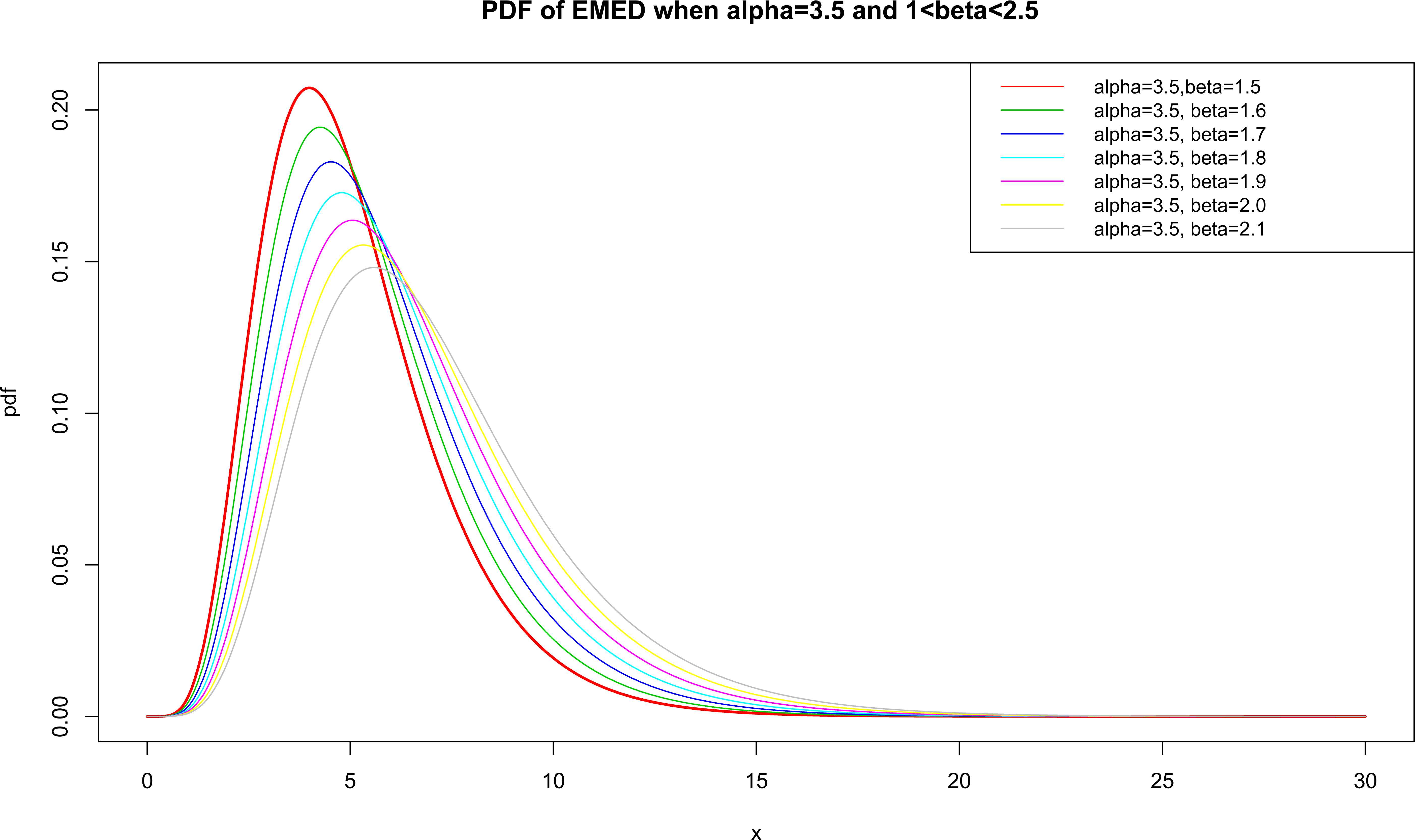
The corresponding reliability function is given by

(1.3)R(x)=1−F(x)=1−[1−x+ββe−xβ]α, x>0,

and the hazard function is

(1.4)h(x)=αβ2 [1−(1+xβ)e−xβ]α−1xe−xβ1−[1−x+ββe−xβ]α; 0<x<∞.

2. Maximum likelihood Estimation for the shape Parameter α of Exponentiated Moment Exponential distribution (EMED) assuming scale parameter β is to be known

Let us consider a random sample x¯=(x1,x2,…,xn) of size n from the Exponentiated Moment Exponential Distribution. Then the likelihood function for the given sample observation is

(2.1)L(x¯|α)=αnβ2n∏i=1n[1−(1+xiβ)e−xiβ]α−1xie−xiβ.

The log-likelihood function is

(2.2)ln L(x¯|α)=n ln α−2n ln β+∑i=1nln xi−1β∑i=1nxi+(α−1)∑i=1nln [1−(1+xiβ)e−xiβ].

As scale parameter β is assumed to be known, the ML estimator of shape parameter α is obtained by solving the

(2.3)∂∂αln L(x¯|α)=0⇒ nα+∑i=1nln [1−(1+xiβ)e−xiβ]=0⇒αˆ=n∑i=1nln [1−(1+xiβ)e−xiβ]−1.

3. The Posterior Distribution of unknown parameter α of Exponentiated Moment Exponential distribution (EMED) using Non-Informative Priors

Bayesian analysis is performed by combining the prior information g(α) and the sample information (x₁,x₂,…,x_n) into what is called the posterior distribution of α given x¯=x1,x2,…,xn from which all decisions and inferences are made. So p(α|x¯) reflects the updated beliefs about α after observing the sample x¯=x1,x2,…,xn.

The posterior distributions using non-informative priors for the unknown parameter α of on exponentiated moment exponential distribution are derived below:

3.1. Posterior Distribution Using Uniform Prior

An obvious choice for the non-informative prior is the uniform distribution. Uniform priors are particularly easy to specify in the case of a parameter with bounded support. The uniform prior of α is defined as:

(3.1)g1(α)∝1, 0<α<∞

The posterior distribution of parameter α for the given data (x¯=x1,x2,…,xn) using (2.1) and (3.1) is:

(3.2)p(α|x¯)∝αnβ2n∏i=1n[1−(1+xiβ)e−xiβ]α−1xie−xiβp(α|x¯)=kαne−α∑i=1nln[1−(1+xiβ)e−xiβ]−1.

Where k is independent of α.

Also, β1=∑i=1nln [1−(1+xiβ)e−xiβ]−1 and k−1=Γ(n+1)β1 n+1.

Therefore from (3.2) we have

(3.3)pU(α|x¯)=β1 n+1Γ(n+1)αne−αβ1;α>0,

which is the density kernel of gamma distribution having parameters α₁ = (n + 1) and β1=∑i=1nln[1−(1+xiβ)e−xiβ]−1. So the posterior distribution of (α|x¯)∼G(α1,β1).

3.2. Posterior Distribution Using Jeffrey’s prior

A non-informative prior has been suggested by Jeffrey’s, which is frequently used in situation where one does not have much information about the parameters. This defines the density of the parameters proportional to the square root of the determinant of the Fisher information matrix, symbolically the Jeffrey’s prior of α is:

g2(α)∝|I(α)|

The Jeffrey’s prior for the shape parameter α of the EMED is derived which is:

(3.4)g2(α)∝1α, 0<α<∞

The posterior distribution of parameter α for the given data (x¯=x1,x2,…,xn) using (2.1) and (3.4) is:

(3.5)p(α|x¯)∝αnβ2n∏i=1n[1−(1+xiβ)e−xiβ]α−1xie−xiβ1αp(α|x¯)=kαn−1e−α∑i=1nln[1−(1+xiβ)e−xiβ]−1,

where k is independent of α, β2=∑i=1nln[1−(1+xiβ)e−xiβ]−1 and k−1=Γ(n)β2 n.

Therefore from (3.5) we have

(3.6)pJ(α|x¯)=β2 nΓ(n)αn−1e−αβ2 ; α>0,

which is the density kernel of gamma distribution having parameters α₂ = n and β2=∑i=1nln[1−(1+xiβ)e−xiβ]−1. So the posterior distribution of (α|x¯)∼G(α2,β2).

4. The Posterior Distribution of unknown parameter αof Exponentiated Moment Exponential distribution (EMED) Using Informative Priors

Here we use gamma and Chi-square distribution as informative prior because they are compatible with the parameter α of the EMED. The posterior distributions using informative priors for the unknown parameter α of the EMED are derived below:

4.1. Posterior Distribution Using Gamma Prior

A way to guarantee that the posterior has an easily calculatable form is to specify a conjugate prior. Conjugacy is a joint property of the prior and the likelihood function that provides a posterior from the same distributional family as the prior. Gamma distribution is the conjugate prior of the EMED. The gamma distribution is used as an informative prior with hyper parameters a and b , having the following p.d.f:

(4.1)g3(α)∝baΓ(a)αa−1e−bα,0<α<∞,a,b>0.

The posterior distribution of parameter α for the given data (x¯=x1,x2,…,xn) using (2.1) and (4.1) is:

(4.2)p(α|x¯)∝αnβ2n∏i=1n[1−(1+xiβ)e−xiβ]α−1xie−xiβbaΓ(a)αa−1e−bαp(α|x¯)=kαn+a−1e−α{b−∑i=1nln[1−(1+xiβ)e−xiβ] },

where k is independent of α, β3={b−∑i=1nln[1−(1+xiβ)e−xiβ] } and k−1=Γ(n+a)β3 (n+a).

Therefore from (4.2) we have

(4.3)pG(α|x¯)=β3 n+aΓ(n+a)αn+a−1e−αβ3; α>0,

which is the density kernel of gamma distribution having parameters α₃ = (n + a) and β3={b−∑i=1nln[1−(1+xiβ)e−xiβ] }. So the posterior distribution of (α|x¯)∼G(α3,β3).

4.2. Posterior Distribution Using Chi-square Prior

Another informative prior is assumed to be the Chi-square distribution with hyper parameter a₂, which has the following p.d.f:

(4.4)g4(α)∝1Γ(a2/2)2a2/2αa22−1e−a22,0<α<∞,a,b>0

The posterior distribution of parameter α for the given data (x¯=x1,x2,…,xn) using (2.1) and (4.4) is:

(4.5)p(α|x¯)∝αnβ2n∏i=1n[1−(1+xiβ)e−xiβ]α−1xie−xiβ1Γ(a2/2)2a2/2αa22−1e−α2p(α|x¯)=kαn+a22−1e−α{12−∑i=1nln[1−(1+xiβ)e−xiβ] },

where k is independent of α, β4={12−∑i=1nln[1−(1+xiβ)e−xiβ] } and k−1=Γ(n+a2/2)β4 (n+a2/2).

Therefore from (4.5) we have

(4.6)pCI(α|x¯)=β4 (n+a2/2)Γ(n+a2/2)αn+a22−1e−αβ4 ;α>0,

which is the density kernel of gamma distribution having parameters α₄ = ((n + a₂)/2) and β4={12−∑i=1nln[1−(1+xiβ)e−xiβ] }. So the posterior distribution of (α|x¯)∼G(α4,β4).

5 Comparison of priors with respect to posterior variances:

The variances of the posterior distribution under all assumed priors is given by

V(α|X)=αiβi 2;i=1,2,3,4.

6. Bayesian estimation of unknown shape parameter α under different loss functions

This section discusses the different Bayes estimators using the loss functions; Squared Error loss function (SELF), Entropy Loss Function (ELF), and precautionary loss function (PLF). While SELF is symmetric, ELF and PLF are asymmetric loss functions:

1.
Squared Error loss function (SELF): A commonly used loss function is the SELF given by
l(αˆ,α)=c(αˆ−α)2,
which is symmetric loss function that assigns equal losses to over estimation and under estimation. The SELF is often used because it does not need extensive numerical computation.
2.
Entropy Loss Function (ELF): The ELF proposed by Calabria and Pulcini (1994) is a useful asymmetric lossfunction given by L(δ^p)∝ [δ^p − p log(δ)−1] where δ=αˆ/α and p>0, whose minimum occur at αˆ=α. Also, this loss function L(δ) has been used by [4] and [5], in the original form having p =1. Thus, L(δ) can be written as
L(δ)=c2[δ−log(δ)−1] ; c2>0.
3.
The Precautionary Loss Function (PLF): [12] introduced an alternative asymmetric precautionary loss function, and also presented a general class of precautionary loss functions as a special case. These loss functions approach infinitely near the origin to prevent under estimation, thus giving conservative estimators, especially when low failure rates are being estimated. A very useful and simple asymmetric precautionary loss function is given by
l(αˆ,α)=(αˆ−α)2αˆ

7. Bayesian Estimation of α under the Assumption of uniform prior

7.1. Estimation under Squared Error loss function

By using squared error loss function l(αˆ,α)=c(αˆ−α)2 for some constant c the risk function is given by

(7.1)R(αˆ,α)=∫0∞c(αˆ−α)2β1 n+1Γ(n+1)αne−αβ1 dα⇒R(αˆ,α)=cβ1 n+1Γ(n+1)[αˆ2Γ(n+1)β1 n+1+Γ(n+3)β1 n+3−2αˆΓ(n+2)β1 n+2].

Now solving ∂∂αˆR(αˆ,α)=0, we obtain the Bayes estimator as αˆUS=(n+1)β1.

7.2. Estimation under Entropy loss function

By using entropy loss function L(δ)=c₂[δ − log δ −1] for some constant c₂ the risk function is given by

(7.2)R(αˆ,α)=∫0∞c2(αˆα−log(αˆα)−1)β1 n+1Γ(n+1)αne−αβ1 dα⇒R(αˆ,α)=c2β1 n+1Γ(n+1)[αˆΓ(n)β1 n−log(αˆ)Γ(n+1)β1 n+1+Γ′(n+1)β1 n+1−Γ(n+1)β1 n+1].

Now solving ∂∂αˆR(αˆ,α)=0, we obtain the Bayes estimator as αˆUEL=nβ1.

7.3. Estimation under precautionary loss function

By using precautionary loss function l(αˆ,α)=(αˆ−α)2αˆ the risk function is given by

(7.3)R(αˆ,α)=∫0∞(αˆ−α)2αˆβ1 n+1Γ(n+1)αne−αβ1 dα⇒R(αˆ,α)=β1 n+1Γ(n+1)[αˆΓ(n+1)β1 n+1+1αˆΓ(n+3)β1 n+3−2Γ(n+2)β1 n+2].

Now solving ∂∂αˆR(αˆ,α)=0, we obtain the Bayes estimator as

αˆUP=[(n+1)(n+2)]1/2β1.

8. Bayesian Estimation of αunder the Assumption of Jeffery’s Prior

8.1. Estimation under Squared Error loss function

By using squared error loss function l(αˆ,α)=c(αˆ−α)2 for some constant c the risk function is given by

(8.1)R(αˆ,α)=∫0∞c(αˆ−α)2β2 nΓ(n)αn−1e−αβ2 dα⇒R(αˆ,α)=cβ2 nΓ(n)[αˆ2Γ(n)β2 n+Γ(n+2)β2 n+2−2αˆΓ(n+1)β2 n+1].

Now solving ∂∂αˆR(αˆ,α)=0, we obtain the Bayes estimator as αˆJS=(n)β2.

8.2. Estimation under Entropy loss function

By using entropy loss function L(δ) = c₂[δ − log δ −1] for some constant c₂ the risk function is given by

(8.2)R(αˆ,α)=∫0∞c2(αˆα−log (αˆα)−1)β2 nΓ(n)αn−1e−αβ2 dα⇒R(αˆ,α)=c2β2 nΓ(n)[αˆΓ(n−1)β2 n−1−log(αˆ)Γ(n)β2 n+Γ′(n)β2 n−Γ(n)β2 n].

Now solving ∂∂αˆR(αˆ,α)=0, we obtain the Bayes estimator as αˆJEL=(n−1)β2.

8.3. Estimation under precautionary loss function

By using precautionary loss function l(αˆ,α)=(αˆ−α)2αˆ the risk function is given by

(8.3)R(αˆ,α)=∫0∞(αˆ−α)2αˆβ2 nΓ(n)αn−1e−αβ2 dα⇒R(αˆ,α)=β2 nΓ(n)[αˆΓ(n)β2 n+1αˆΓ(n+2)β2 n+2−2Γ(n+1)β2 n+1].

Now solving ∂∂αˆR(αˆ,α)=0, we obtain the Bayes estimator as

αˆJP=[(n)(n+1)]1/2β2.

9. Bayesian Estimation of α under the Assumption of Gamma Prior

9.1. Estimation under Squared Error loss function

By using squared error loss function l(αˆ,α)=c(αˆ−α)2 for some constant c the risk function is given by

(9.1)R(αˆ,α)=∫0∞c(αˆ−α)2β3 n+aΓ(n+a)αn+a−1e−αβ3 dα⇒R(αˆ,α)=cβ3 n+aΓ(n+a)[αˆ2Γ(n+a)β3 n+a+Γ(n+a+2)β3 n+a+2−2αˆΓ(n+a+1)β3 n+a+1].

Now solving ∂∂αˆR(αˆ,α)=0, we obtain the Bayes estimator as αˆGS=(n+a)β3.

9.2. Estimation under Entropy loss function

By using entropy loss function L(δ) = c₂[δ − log δ −1] for some constant c₂ the risk function is given by

(9.2)R(αˆ,α)=∫0∞c2(αˆα−log(αˆα)−1)β3 n+aΓ(n+a)αn+a−1e−αβ3 dα⇒R(αˆ,α)=c2β3 n+aΓ(n+a)[αˆΓ(n+a−1)β3 n+a−1−log(αˆ)Γ(n+a)β3 n+a+Γ′(n+a)β3 n+a−Γ(n+a)β3 n+a].

Now solving ∂∂αˆR(αˆ,α)=0, we obtain the Bayes estimator as

αˆGEL=(n+a−1)β3.

9.3. Estimation under precautionary loss function

By using precautionary loss function l(αˆ,α)=(αˆ−α)2αˆ the risk function is given by

(9.3)R(αˆ,α)=∫0∞(αˆ−α)2αˆβ3 n+aΓ(n+a)αn+a−1e−αβ3 dα⇒R(αˆ,α)=β3 n+aΓ(n+a)[αˆΓ(n+a)β3 n+a+1αˆΓ(n+a+2)β3 n+a+2−2Γ(n+a+1)β3 n+a+1].

Now solving ∂∂αˆR(αˆ,α)=0, we obtain the Bayes estimator as

αˆGP=[(n+a)(n+a+1)]1/2β3.

10. Bayesian Estimation of α under the Assumption of Chi-square Prior

10.1. Estimation under Squared Error loss function

By using squared error loss function l(αˆ,α)=c(αˆ−α)2 for some constant c the risk function is given by

(10.1)R(αˆ,α)=∫0∞c(αˆ−α)2β4 (n+a2/2)Γ(n+a2/2)αn+a22−1e−αβ4 dα⇒R(αˆ,α)=cβ4 (n+a2/2)Γ(n+a2/2)[αˆ2Γ(n+a2/2)β4 (n+a2/2)+Γ(n+a2/2+2)β4 (n+a2/2+2)−2αˆΓ(n+a2/2+1)β4 (n+a2/2+1)]

Now solving ∂∂αˆR(αˆ,α)=0, we obtain the Bayes estimator as

αˆCIS=(n+a2/2)β4.

10.2. Estimation under Entropy loss function

By using entropy loss function L(δ) = c₂[δ − log δ −1] for some constant c₂ the risk function is given by

(10.2)R(αˆ,α)=∫0∞c2(αˆα−log(αˆα)−1)β4 (n+a2/2)Γ(n+a2/2)αn+a22−1e−αβ4 dα⇒R(αˆ,α)=c2β4 (n+a2/2)Γ(n+a2/2)[αˆΓ(n+a2/2)β4 n+a2/2−1−log(αˆ)Γ(n+a2/2)β4 n+a2/2+Γ′(n+a2/2)β4 n+a2/2−Γ(n+a2/2)β4 n+a2/2]

Now solving ∂∂αˆR(αˆ,α)=0, we obtain the Bayes estimator as

αˆCIEL=(n+a2/2−1)β4.

10.3. Estimation under precautionary loss function

By using precautionary loss function l(αˆ,α)=(αˆ−α)2αˆ, the risk function is given by

(10.3)R(αˆ,α)=∫0∞(αˆ−α)2αˆβ4 (n+a2/2)Γ(n+a2/2)αn+a22−1e−αβ4 dα⇒R(αˆ,α)=β4 (n+a2/2)Γ(n+a2/2)[αˆΓ(n+a2/2)β4 (n+a2/2)+1αˆΓ(n+a2/2+2)β4 (n+a2/2+2)−2Γ(n+a2/2+1)β4 (n+a2/2+1)].

Now solving ∂∂αˆR(αˆ,α)=0, we obtain the Bayes estimator as

αˆCIP=[(n+a2/2)(n+a2/2+1)]1/2β4.

11. Applications

To compare the performance of the estimates under differentloss functions for the exponentiated moment exponential distribution, two real data sets are used and analysis performed with the help of R software.

Data set I: The first data set consists of 100 observations on breaking stress of carbon fibers (in Gba). The data has been previously used by [11], the data is as follows:

3.70, 2.74, 2.73, 2.50, 3.60, 3.11, 3.27, 2.87, 1.47, 3.11, 4.42, 2.41, 3.19, 3.22, 1.69, 3.28, 3.09, 1.87, 3.15, 4.90, 3.75, 2.43, 2.95, 2.97, 3.39, 2.96, 2.53, 2.67, 2.93, 3.22, 3.39, 2.81, 4.20, 3.33, 2.55, 3.31, 3.31, 2.85, 2.56, 3.56, 3.15, 2.35, 2.55, 2.59, 2.38, 2.81, 2.77, 2.17, 2.83, 1.92, 1.41, 3.68, 2.97, 1.36, 0.98, 2.76, 4.91, 3.68, 1.84, 1.59, 3.19, 1.57, 0.81, 5.56, 1.73, 1.59, 2.00, 1.22, 1.12, 1.71, 2.17, 1.17, 5.08, 2.48, 1.18, 3.51, 2.17, 1.69, 1.25, 4.38, 1.84, 0.39, 3.68, 2.48, 0.85, 1.61, 2.79, 4.70, 2.03, 1.80, 1.57, 1.08, 2.03, 1.61, 2.12, 1.89, 2.88, 2.82, 2.05, 3.65

β	MLE	SELF	ELF	PLF
3.0	0.59076	0.59667	0.59076	0.59962
3.5	0.51957	0.52476	0.51957	0.52735
4.0	0.46866	0.47335	0.46866	0.47569
4.5	0.43033	0.43463	0.43033	0.43678

Table 1.

Bayes Estimates of α under Uniform Prior

β	MLE	SELF	ELF	PLF
3.0	0.59076	0.59076	0.58485	0.59371
3.5	0.51957	0.51957	0.51437	0.52216
4.0	0.46866	0.46866	0.46398	0.47100
4.5	0.43033	0.43033	0.42603	0.43248

Table 2.

Bayes Estimates of α under Jeffrey Prior

β	a	b	MLE	SELF	ELF	PLF
3.0	1.4	0.4	0.59076	0.59762	0.59173	0.60056
3.5	1.4	0.4	0.51957	0.52575	0.52056	0.52833
4.0	1.4	0.4	0.46866	0.47433	0.46966	0.47666
4.5	1.4	0.4	0.43033	0.43561	0.43131	0.43775

Table 3.

Bayes Estimates of α under Gamma Prior

β	a₂	MLE	SELF	ELF	PLF
3.0	0.3	0.59076	0.58991	0.58401	0.59284
3.5	0.3	0.51957	0.51900	0.51381	0.52158
4.0	0.3	0.46866	0.46827	0.46359	0.47060
4.5	0.3	0.43033	0.43005	0.42576	0.43219

Table 4.

Bayes Estimates of α under Chi-square Prior

From tables 5 to 8 we conclude that squared error loss function provides the minimum posterior risk as compared to the other loss functions particularly as loss parameter C is (0.5) and among the priors Chi-square prior provides the less posterior risk than other priors.

β	SELF		ELF		PLF

	C=0.5	C=1.0	C₂=0.5	C₂=1.0
3.0	0.00176	0.00352	2.56825	5.13650	0.00589
3.5	0.00136	0.00272	2.63245	5.26491	0.00518
4.0	0.00111	0.00222	2.68402	5.36803	0.00468
4.5	0.00093	0.00187	2.72667	5.45335	0.00429

Table 5.

Bayes Risk of α under Uniform Prior

β	SELF		ELF		PLF

	C=0.5	C=1.0	C₂=0.5	C₂=1.0
3.0	0.00174	0.00349	2.56827	5.13655	0.00589
3.5	0.00135	0.00269	2.63248	5.26496	0.00518
4.0	0.00109	0.00219	2.68404	5.36808	0.00467
4.5	0.00092	0.00185	2.72670	5.45340	0.00429

Table 6.

Bayes Risk of α under Jeffrey Prior

β	a	b	SELF		ELF		PLF

			C=0.5	C=1.0	C₂=0.5	C₂=1.0
3.0	1.4	0.4	0.00176	0.00352	2.56942	5.13884	0.00588
3.5	1.4	0.4	0.00136	0.00272	2.63348	5.26697	0.00517
4.0	1.4	0.4	0.00111	0.00222	2.68494	5.36988	0.00467
4.5	1.4	0.4	0.00093	0.00187	2.72752	5.45505	0.00428

Table 7.

Bayes Risk of α under Gamma Prior

β	a₂	SELF		ELF		PLF

		C=0.5	C=1.0	C₂=0.5	C₂=1.0
3.0	0.3	0.00174	0.00347	2.56975	5.13949	0.00588
3.5	0.3	0.00134	0.00268	2.63377	5.26755	0.00516
4.0	0.3	0.00109	0.00219	2.68521	5.37042	0.00466
4.5	0.3	0.00092	0.00185	2.72777	5.45554	0.00429

Table 8.

Bayes Risk of α under Chi-square Prior

Data set II: The second data - set represents the waiting times (in minutes) before service of 100 Bank customers and examined and analyzed by [7] for fitting [10] the Lindley distribution. The data are as follows:

0.8, 0.8, 1.3, 1.5, 1.8, 1.9, 1.9, 2.1, 2.6, 2.7, 2.9, 3.1, 3.2, 3.3, 3.5, 3.6, 4.0, 4.1, 4.2, 4.2, 4.3, 4.3, 4.4, 4.4, 4.6, 4.7, 4.7, 4.8, 4.9, 4.9, 5.0, 5.3, 5.5, 5.7, 5.7, 6.1, 6.2, 6.2, 6.2, 6.3, 6.7, 6.9, 7.1, 7.1, 7.1, 7.1, 7.4, 7.6, 7.7, 8.0, 8.2, 8.6, 8.6, 8.6, 8.8, 8.8, 8.9, 8.9, 9.5, 9.6, 9.7, 9.8, 10.7, 10.9, 11.0, 11.0, 11.1, 11.2, 11.2, 11.5, 11.9, 12.4, 12.5, 12.9, 13.0, 13.1, 13.3, 13.6, 13.7, 13.9, 14.1, 15.4, 15.4, 17.3, 17.3, 18.1, 18.2, 18.4, 18.9, 19.0, 19.9, 20.6, 21.3, 21.4, 21.9, 23.0, 27.0, 31.6, 33.1, 38.5.

β	MLE	SELF	ELF	PLF
3.0	1.78893	1.80682	1.78893	1.81574
3.5	1.47874	1.49353	1.47874	1.50090
4.0	1.26545	1.27810	1.26545	1.28441
4.5	1.11063	1.12173	1.11063	1.12727

Table9.

Bayes Estimates of α under Uniform Prior

β	MLE	SELF	ELF	PLF
3.0	1.78893	1.78893	1.77104	1.79785
3.5	1.47874	1.47874	1.46395	1.48611
4.0	1.26545	1.26545	1.25279	1.27176
4.5	1.11063	1.11063	1.09952	1.11617

Table 10.

Bayes Estimates of α under Jeffrey Prior

β	a	b	MLE	SELF	ELF	PLF
3.0	1.4	0.4	1.78893	1.80109	1.78332	1.80995
3.5	1.4	0.4	1.47874	1.49062	1.47592	1.49796
4.0	1.4	0.4	1.26545	1.27670	1.26411	1.28298
4.5	1.4	0.4	1.11063	1.12119	1.11014	1.12671

Table11.

Bayes Estimates of α under Gamma Prior

β	a₂	MLE	SELF	ELF	PLF
3.0	0.3	1.78893	1.77573	1.75800	1.78457
3.5	0.3	1.47874	1.47009	1.45541	1.47741
4.0	0.3	1.26545	1.25938	1.24680	1.26565
4.5	0.3	1.11063	1.10615	1.09510	1.11166

Table12.

Bayes Estimates of α under Chi-square Prior

From tables 13 to 16 we conclude that squared error loss function provides the minimum posterior risk as compared to the other loss functions particularly as loss parameter C is (0.5) and among the priors Chi-square prior provides the less posterior risk than other priors.

β	SELF		ELF		PLF

	C=0.5	C=1.0	C₂=0.5	C₂=1.0
3.0	0.01616	0.03232	2.01427	4.02854	0.01784
3.5	0.01104	0.02208	2.10948	4.21897	0.01475
4.0	0.00808	0.01617	2.18736	4.37473	0.01262
4.5	0.00623	0.01245	2.25261	4.50523	0.01107

Table13.

Bayes Risk of α under Uniform Prior

β	SELF		ELF		PLF

	C=0.5	C=1.0	C₂=0.5	C₂=1.0
3.0	0.01600	0.03200	2.01429	4.02859	0.01784
3.5	0.01093	0.02186	2.10951	4.21902	0.01475
4.0	0.00801	0.01601	2.18739	4.37478	0.01262
4.5	0.00616	0.01233	2.25264	4.50528	0.01107

Table14.

Bayes Risk of α under Jeffrey Prior

β	a	b	SELF		ELF		PLF

			C=0.5	C=1.0	C₂=0.5	C₂=1.0
3.0	1.4	0.4	0.01599	0.03199	2.01782	4.03565	0.01771
3.5	1.4	0.4	0.01095	0.02191	2.11242	4.22484	0.01466
4.0	1.4	0.4	0.00803	0.01607	2.18988	4.37976	0.01255
4.5	1.4	0.4	0.00619	0.01239	2.25482	4.50964	0.01103

Table15.

Bayes Risk of α under Gamma Prior

β	a₂	SELF		ELF		PLF

		C=0.5	C=1.0	C₂=0.5	C₂=1.0
3.0	0.3	0.01574	0.03148	2.01874	4.03749	0.01768
3.5	0.3	0.01078	0.02157	2.11319	4.22637	0.01464
4.0	0.3	0.00791	0.01583	2.19054	4.38108	0.01254
4.5	0.3	0.00611	0.01221	2.25540	4.51081	0.01101

Table16.

Bayes Risk of α under Chi-square Prior

12. Conclusion

On comparing the Bayes posterior risk of different loss functions, it is observed that SELF has less Bayes posterior risk than other loss functions in both non informative and informative priors. According to the decision rule of less Bayes posterior risk we conclude that SELF is more preferable loss function for different values of α.

It is clear from Tables 5 to 8 and Tables 13 to 16, the comparison of Bayes posterior risk under different loss functions using non-informative as well as informative priors has been made through which we conclude that within each loss function informative. Chi-square prior provides less Bayes posterior risk than other priors so it is more suitable for the exponentiated moment exponential distribution.

Acknowledgements

The authors are highly grateful to the Editor and referees for their constructive comments and suggestions that greatly improved the manuscript.

References

[1]Afaq Ahmad, SP Ahmad, and A Ahmed, Preference of priors for the exponentiated exponential distribution under different loss functions, International Journal of Modern Mathematical Sciences, Vol. 13, No. 3, 2015, pp. 307-321.

[2]R Calabria and G Pulcini, An engineering approach to Bayes estimation for the Weibull distribution, Microelectronics Reliability, Vol. 34, No. 5, 1994, pp. 789-802.

[3]ST Dara and M Ahmad, Recent Advances in Moment Distributions and their Hazard Rate, Ph.D. Thesis”, National College of Business Administration and Economics, Lahore, Pakistan, 2012.

[4]DK Dey, M Ghosh, and C Srinivasan, Simultaneous Estimation of Parameters under Entropy loss, J. Statist. Plan. and Infer, 1987, pp. 347-363.

[5]DK Dey and Pie-San L Liu, On Comparison of Estimators in a Generalized Life Model, Micro-electron. Reliab, Vol. 45, No. 3, 1992, pp. 207-221.

[6]ZSM Farahani and E Khorram, Bayesian statistical inference for weighted exponential distribution, Communicationsin Statistics-Simulation and Computation, Vol. 43, 2014, pp. 1362-1384.

[7]ME Ghitany, B Atieh, and S Nadarajah, Lidley distribution and its Application, Mathematics Computing and Simulation, Vol. 78, 2008, pp. 493-506.

[8]RD Gupta and D Kundu, A new class of weighted exponential distribution, Statistics, Vol. 43, No. 6, 2009, pp. 621-634.

[9]SA Hasnain, Exponentiated Moment Exponential Distribution, Ph.D. Thesis, National College of Business Administration and Economics, Lahore, Pakistan, 2013.

[10]D Lindley, Fiducial distributions and Bayes’ theorem, journal of the Royal Statistical Society, Vol. 20, No. 1, 1958, pp. 102-107.

[11]MD Nichols and WJ Padgett, A Bootstrap control chart for Weibull percentiles, Quality and Reliability Engineering International, Vol. 22, 2006, pp. 141-151.

[12]JG Norstrom, The use of precautionary loss function in risk analysis, IEEE Transactions on Reliability, Vol. 45, No. 3, 1996, pp. 400-403.

[13]Sofi Mudasir, SP Ahmad, and A Ahmad, Bayesian Estimation of Length Biased Nakagami Distribution, International Journal of Modern Mathematical Sciences, Vol. 14, No. 2, 2016, pp. 147-159.

<Previous Article In Issue

Download article (PDF)

Next Article In Issue>

Journal: Journal of Statistical Theory and Applications
Volume-Issue: 17 - 2
Pages: 359 - 374
Publication Date: 2018/06/30
ISSN (Online): 2214-1766
ISSN (Print): 1538-7887
DOI: 10.2991/jsta.2018.17.2.13 How to use a DOI?
Open Access: This is an open access article under the CC BY-NC license (http://creativecommons.org/licences/by-nc/4.0/).

Cite this article

ris enw bib

TY  - JOUR
AU  - Kawsar Fatima
AU  - S.P Ahmad*
PY  - 2018
DA  - 2018/06/30
TI  - BAYESIAN APPROACH IN ESTIMATION OF SHAPE PARAMETER OF THE EXPONENTIATED MOMENT EXPONENTIAL DISTRIBUTION
JO  - Journal of Statistical Theory and Applications
SP  - 359
EP  - 374
VL  - 17
IS  - 2
SN  - 2214-1766
UR  - https://doi.org/10.2991/jsta.2018.17.2.13
DO  - 10.2991/jsta.2018.17.2.13
ID  - Fatima2018
ER  -

download .riscopy to clipboard