
Joint Modeling of Linear Degradation and Multiple Dependent Competing Risks Data under a Step-Stress Accelerated Degradation Test
- DOI
- 10.2991/jsta.2018.17.2.12How to use a DOI?
- Keywords
- Dependent Competing Risk; Copula Function; Reliability Function; Step-Stress Accelerated Degradation Test
- Abstract
The step-stress accelerated degradation test (SSADT) is one of the most commonly used time-dependent types of stress loading tests that enables a shorter test duration. This test is more economical and flexible compared to accelerated degradation test or accelerated failure time (ADT/AFT) test plans. This test is suitable when constraints by test facilities, conditions, or samples exist. SSADT is more useful for developing products when there is inadequate knowledge for test conditions. Important aspects here are to evaluate each failure mode in the presence of the other modes by assuming some dependency structure between the failure modes due to the non-applicability of studying test units with isolated competing failure modes. This paper aims to propose a modeling approach to simultaneously analyze linear degradation data and failure time data with dependent competing risks in an SSADT experiment. We use the copula function to consider the dependency structures between two failure modes. The proposed model is applied to acceleration data, to simulation data sets and two real data sets- bus tire data set and plastic substrate active matrix light-emitting diodes (AMOLED) data set, accompanied by sensitivity analysis.
- Copyright
- Copyright © 2018, the Authors. Published by Atlantis Press.
- Open Access
- This is an open access article under the CC BY-NC license (http://creativecommons.org/licences/by-nc/4.0/).
1. Introduction
The development of engineering and science technology have led to increased public awareness and insistence on product quality, in addition to consumer production laws and regulations that concern product reliability and profit consideration from the high costs of failures, repairs, and warranty programs. Hence, the products become increasingly more reliable, with an extended product life.
Under these circumstances it is difficult to assess product reliability according to traditional life-testing procedures based solely on time to failure under normal operation conditions. It is more difficult to obtain sufficient time to failure data to estimate their lifetime efficiency.
In order to overcome this difficulty, reliability practitioners have attempted to design methods that obtain failures quickly by exposing the products to acute environmental conditions without the introduction of additional failure modes other than those observed under normal conditions. The term accelerated life testing (ALT) describes these methods. ALT models can be categorized to accelerated failure time (AFT) model where stresses take effect on the failure time multiplicatively, the proportional odds (PO) model [3] that stresses take effect on an increased odds of failure rate, the proportional hazard (PH) model [6] in which stresses take effect on the failure rate multiplicatively, the extended hazard regression (EHR) model [5], the extended linear hazard regression (ELHR) model [7], in which both AFT and PH models are incorporated, and the proportional odds (PO) model [3] that stresses take effect on an increased odds of failure rate. Although ALT assesses the lifetime characteristics of the components with high reliability, this procedure may involve the collection of only a few failures.
To handle this problem, accelerated degradation testing (ADT) is considered as an alternative method. ADT combines degradation testing with ALT by means of testing the products in harsh environments and measuring the degradation of products during the acceleration test. In contrast to the ALT method in which the failure time is recorded, in the ADT method, both the failure information and degradation information may be obtained. As a result, the product reliabilities can be estimated more accurately. However, this method is generally very costly and usually requires a moderate sample size to be implemented. The ADT method also has its own difficulties in terms of not being applicable for evaluating the lifetime of a newly developed or a very expensive product with a few available units at hand. As a result, and to ensure enough failed units in a limited testing period, it is more realistic to consider multiple stress-type accelerated life testing methods. Most previous literature that discuss designing ALT/ADT plans have focused on the application of a single stress type, which usually requires a long test duration, complicated stress level selection process, large sample sizes, and high test costs. Literature about designing an ADT began at the end of the last century. Key references that pertain to ALT and ADT include [19], [23] and [26].
Under this situation, a constant stress ADT is not applicable. Tseng et al. [30] have proposed a step stress ADT (SSADT). In this accelerated life testing all samples are tested together under step stresses, which lead to a shorter test duration and the need for a smaller sample size. SSALT/SSADT is often preferred to constant stress ALT/ADT because it can avoid a high stress start point and possibly additional, unrelated failure modes. Concise reviews of SSALT have been presented by Nelson [19]. Liao [14] discussed how to efficiently design a SSADT experiment with an optimal sample size and termination time. Numerous papers have been published following the gradual development of degradation models. Park et al. [24] studied the optimum method of SSADT in the case of destructive measurement. More general time-varying-stress ALTs were considered by [12] and [2]. Turner [31], as well as Fan and Wang [10], discussed the statistical analysis of ALTs. Peng et al. [25] reported a model-based review of SSADT in terms of gradual development and improvement of degradation models which were categorized as degradation path models and Markovian models [17], and stochastic process based models [20].
Due to the existence of competing failure modes and non-applicability of studying test units with isolated competing failure modes, it is necessary to evaluate each failure mode in the presence of other modes by assuming some dependency structure between the failure modes. Recently, most researches of SSADT plans are based on an underlying assumption of one mode of failure. However, due to the complexity of high reliable products, their reliability should be evaluated by more than one mode of failure. Few works have focused on multiple degradation mechanisms or general multiple mechanism failure. Overviews of joint modeling of failure times and degradation data, as well as design problems have been discussed by [11], [15] and [21]. Liu and Qiu [16] proposed a method for planning multiple step-stress ALT with competing risks. Pan and Sun [22] presented an SSADT model with two performance characteristics based on gamma processes. Of note, in these SSADT models, a common but unrealistic assumption of researchers is the independency of the failure modes. However if the assumption of independence is violated, then the result may not be trustworthy and could result in an inaccurate estimation of the products lifetime. In this paper, we have extended the SSADT model proposed by Haghighi and Bae [11] in order to estimate reliability function in the presence of dependent competing risks.
Numerous researchers have applied the copula method to the dependence analysis of competing failures in the SSALT method (However this has not been studied in SSADT.). Simon and Wilke [27] presented an approach to the estimation of a nonparametric competing risk duration model based on an assumed dependence structure and illustrated the framework by analyzing the effect of reduced unemployment benefit entitlements on the duration of unemployment in Germany. Eryilmaz [8] studied the problem of estimating the parameter of the common distribution of component lifetime from a system lifetime data. It was assumed that the common component distribution was exponential, and that the component lifetimes were dependent through a completely known exchangeable Archimedean copula. Few studies reported the statistics for ALT with dependent competing failures. Although Xu and Tang [32] performed a pilot study on the statistics for ALT on the basis of the copula, this study was only a special case with an exponential distribution of all the competing failure modes; the copula was assumed to be a Gumbel copula, not a study with more general applications.
As previously mentioned, failure modes are usually dependent because of coupling factors such as running under the same working conditions. Therefore, the assumption that all the competing failure modes are independent is not true in practice. The statistics of SSADT based on this assumption may lead to incorrect results for product lifetime and reliability. However this has not been studied. In this paper, we propose a modeling approach for jointly analyzing linear degradation data and dependent failure times simultaneously recorded during the SSADT. Under the modeling approach, a step-stress accelerated test has been taken into account for unit failures with dependent multiple modes (competing risks). In each level of stress under the SSADT, we assume that failure times, their failure modes, and the amount of degradation at the moment of failures are recorded for failed units. For the units that have not failed at the end of each step-stress, only the amount of degradation is recorded. We apply the copula model to combine the marginal distribution of the competing failure models with the time to failure distribution of the products, and derived a general statistical model for SSADT with dependent competing failures. It is widely believed that the copula method is the most convenient and important tool for solving dependence problems. Finally, we have derived a likelihood function for failure-times from degradation data to provide maximum likelihood estimates (MLEs) of the parameters of the proposed model and the reliability function.
This paper is organized as follows. In Section two, we describe the copula functions, the competing risks framework in the SSADT method and express the likelihood and reliability funcrion. In Section three, we provide three examples from simulation and real data in an attempt to compare the efficiency of the SSADT plan proposed in this paper considering dependency between failure modes using the copula functions and that given by [11]. In Section four we have performed sensitivity analysis for the effect of chaning the copula function and the change-point of the stress on parameter estimation under a simple SSADT. Finally, conclusion and possible directions for future study are discussed in Section five.
2. The proposed model
This section is divided into three subsections. In the first subsection, we briefly explain the concept of copula function and in the second subsection, we discuss SSADT in the competing risks framework and give likelihood function in this method. In the third subsection, we describe a methodology for step-stress reliability function.
2.1. Copula Function
There is a need for more realistic modeling of a stochastic dependency structure that contain all information about dependent random variables, which goes beyond the measure of linear correlation coefficients and has the capability to capture co-dependency outside the world of elliptical distributions, particularly in situations where marginal functions are known and joint distributions may be unknown. Alternative methods for capturing co-dependency have been considered. One class of alternatives is the copula-based dependencies that have been introduced in statistical literature by [28]. This approach allows one to model the dependence structure independently of marginal distributions. This approach provides an alternative and frequently more useful representation of multivariate distribution compared to traditional approaches such as multivariate normality. Note that an independent copula implies zero correlation but the opposite is false. Joe [13] and Nelsen [18] have discussed this more thoroughly.
Formally, copulas can be defined as follows. Suppose that we have two marginal CDFs, GX1(x1), FX2(x2) where X1, X2 are the random variables. Sklar’s theorem states that every bivariate cumulative distribution function
The random variables X1 and X2 are said to be independent if:
According to Sklar’s canonical representation, if R be a 2-dimensional survival function with margins R1,R2, then R has a copula representation:
There are some 1-parameter copulas that can be used. For example: the elliptical family (i.e. Gaussian, t) and Archimedean family (i.e. Frank, Gumbel, Clayton). One of the popular Archimedean copulas is the Frank copula. It is a symmetric copula (for bivariate data) given by
Its generator is:
- 1)
It has a simple closed form with one parameter.
- 2)
It includes positive and negative dependency.
- 3)
It has symmetric dependence.
In this paper, we use the Frank copula to describe the dependence of the degradation and hard failure time. Č and C are equal in Frank copula. This dependency can be measured using copula parameter θ. There is an explicit relation between the Kendall’s tau and the parameter of Frank copula (θ). Specifically,
The relations between copula parameter, θ, correlation coefficient, ρ, and Kendalls tau, τθ, are given for some values of θ in Table 1.
| θ = −1 | τθ = −0.1100185 | ρ = −0.1644861 |
| θ = −200 | τθ = −0.9801645 | ρ = −0.9995137 |
Relation between copula parameter and correlation coefficients
2.2. The competing risks framework in the SSADT method
To express the framework of competing risks in SSADT, we must initially explain the concept of SSADT. Suppose that degradation models are linear and the rate of degradation depends only on current stress [30]. Although linear degradation has been considered by numerous authors, including [29], it appears that the simultaneous analysis of degradation and failure-time data with multiple failure modes is rare, especially when failure modes are dependent. This is attributed to the fact that inference on the parameters in the joint model is complicated under an SSADT. The inference procedure under the linear degradation model can be adapted to more general degradation models under an SSADT. In this section, we use a cumulative exposure model for SSADT data. This model is presented in [19].
Let n units be placed on the test. The testing time starts in τ0 = 0. All of the units are first subjected to a normal stress, S0. Afterwards, at changing time stress τ1, all surviving units are moved to the stress level S1 until time τ2. The stress on a unit is thus increased step by step until it fails. So, we have a sequence of changing time points of stress τi,i = 0,…,m + 1. The levels of stresses, S, can be expressed as:
As previously mentioned, we consider the linear degradation process: {Z(t);t > 0} as Z(t) = t/A,A ∈ R, where A is a random variable with a distribution function of FA(a; η) for the q-dimensional vector of parameters η, which is influenced by stress levels. As a result, a density function of A under the SSADT can be written as:
Let Tij be the failure time of i-th level of stress for the j-th unit, where i = 1,…,m and j = 1,…,ni and Zijs be degradation values at time Tij. Suppose we have s failure modes at each level of stress. Therefore failure time is defined as:
Under SSADT, we observe the data set {Tij,Vij,Zij}. Suppose that the rates of failures corresponding to different failure mechanisms are increasing functions of degradation values (e.g., [15]). Let
Under a cumulative exposure model in a SSADT ( [30]) the failure time at time t under the i-th level of stress due to the k-th failure mode has an equivalent failure-time, denoted by t⋆. This would be the time that produces the same amount of cumulative degradation under normal stress. Thus, the equivalent failure-time under normal stress t⋆ is a solution of the equation:
The equivalent failure-time t⋆ at normal stress S0 is derived from (2.4) and (2.5) as:
According to [11], the failure rate at time t and the conditional reliability function corresponding to the k-th failure mode are given by:
Let T = min(T1,..,Ts) be the failure time of unit under dependent competing risks. Our goal is to model the reliability function of T. Denote the reliability function by RT(.). We have:
When failure modes are dependent, we use the crude hazard function (λ(k)(t)) instead of marginal hazard function (λk(t)). The crude hazard function known as the ’cause-specific hazard rate’, is defined as:
Analysis of reliability function requires that we choose a class of copulas. We use Franks family of copulas.
According to (2.9) and (2.10), the crude density functions can then be written as:
As mentioned earlier, λk(t) and λ(k)(t) do not coincide when failure modes are dependent. From (2.8) and (2.9), we can obtain the relation between them as following:
From the observed data at the end of each step of test and (2.8), (2.11) and (2.13), the likelihood function is obtained as the following form:
The MLEs of
When we ignore the dependency between failure modes, the likelihood function changes to:
In order to prove the identifiability of likelihood function L, we show the identifiability of
2.3. Step-Stress Reliability Function
The unconditional reliability (survival) function can be defined as:
Thus the estimate of reliability function is:
3. Examples
3.1. Simulation Study
In order to illustrate the proposed method, we generated n data sets under SSADT by considering a simple step-stress test with a changing time point of τ1 = 40. We suppose that the failure rates of two failure modes depends on the amount of degradation as λk(z(t)) = (θkz(t))νk for k = 1,2. In addition, we assume that the distribution of A in Z = t/A is Weibull with parameters α = 5 and β = 4.
For different sample sizes n = 30,50,80,200, given parameter values θ1 = 0.06, ν1 = 5, θ2 = 0.06 and ν2 = 5, we generated n random samples with B = 1000 replications based on the following steps. We consider the dependency between failure modes using Frank copula with parameter θ = 20.
- Step 1:
Generate random sample U of size n, where U ∼ Uniform(0,1).
- Step 2:
Transform U, into the failure times T, based on the equation (2.12):
where R1,R2 are the marginal reliability function of T1,T2. - Step 3:
Generate random sample A of size n, where A ∼ Weibull(5,4).
- Step 4:
Transform A, into the degradation Z, based on Z = T/A.
Then, we transform data in normal use into the accelerated data with a changing time point of τ1 = 40. Let a0j,a1j denote the values of A for the j-th unit at the first (normal) and second level of stress. We observe a0j according to linear degradation path as t0j/z0j, where t0j, and z0j are failure time and degradation of j-th unit at normal stress, but a1j has been generated from a Weibull distribution with parameters α = 8, β = 5.5. From (2.6) and simulated a1j, the failure times in second level of stress can be computed.
The estimation of parameters of failure rates (θ1, ν1, θ2, ν2), the parameters of Ai, (α0, β0), and the copula parameter, θ, have been obtained using a numerical solution of the likelihood functions (2.14) and (2.15). Table 2 shows estimation results in two cases: independent and dependent failure modes. The estimated median of the lifetime
| Dependent | Independent | ||||||
|---|---|---|---|---|---|---|---|
| n | Param. | Estimate | SE | MRE | Estimate | SE | MRE |
| n=30 | α0 | 5.149 | 0.774 | 0.130 | 5.149 | 0.774 | 0.130 |
| β0 | 3.964 | 0.161 | 0.031 | 3.964 | 0.161 | 0.031 | |
| θ1 | 0.059 | 0.009 | 0.105 | 0.038 | 0.026 | 0.403 | |
| ν1 | 5.411 | 1.199 | 0.193 | 4.006 | 2.502 | 0.426 | |
| θ2 | 0.060 | 0.006 | 0.080 | 0.035 | 0.025 | 0.424 | |
| ν2 | 5.626 | 1.262 | 0.216 | 3.663 | 2.319 | 0.405 | |
| θ | 13.18 | 13.42 | 0.595 | - | - | - | |
| τθ | 0.734 | - | 0 | - | - | ||
| M | 38.76 | - | - | 41.34 | - | - | |
| n=50 | α0 | 5.139 | 0.572 | 0.092 | 5.139 | 0.572 | 0.092 |
| β0 | 3.996 | 0.114 | 0.023 | 3.996 | 0.114 | 0.023 | |
| θ1 | 0.059 | 0.005 | 0.067 | 0.037 | 0.024 | 0.399 | |
| ν1 | 5.228 | 0.893 | 0.136 | 3.628 | 2.193 | 0.389 | |
| θ2 | 0.059 | 0.005 | 0.068 | 0.039 | 0.023 | 0.345 | |
| ν2 | 5.208 | 0.873 | 0.136 | 3.953 | 2.151 | 0.348 | |
| θ | 16.33 | 12.45 | 0.547 | - | - | - | |
| τθ | 0.779 | - | 0 | - | - | ||
| M | 38.35 | - | - | 40.08 | - | - | |
| n=80 | α0 | 5.098 | 0.468 | 0.073 | 5.098 | 0.468 | 0.073 |
| β0 | 3.995 | 0.096 | 0.019 | 3.995 | 0.096 | 0.019 | |
| θ1 | 0.059 | 0.004 | 0.057 | 0.037 | 0.024 | 0.390 | |
| ν1 | 5.151 | 0.673 | 0.104 | 3.594 | 2.082 | 0.362 | |
| θ2 | 0.059 | 0.004 | 0.055 | 0.040 | 0.023 | 0.338 | |
| ν2 | 5.186 | 0.683 | 0.108 | 3.937 | 2.072 | 0.322 | |
| θ | 16.59 | 12.27 | 0.536 | - | - | - | |
| τθ | 0.782 | - | - | 0 | - | - | |
| M | 38.13 | - | - | 39.74 | - | - | |
| n=200 | α0 | 5.048 | 0.278 | 0.044 | 5.048 | 0.278 | 0.044 |
| β0 | 4.000 | 0.061 | 0.012 | 4.000 | 0.061 | 0.012 | |
| θ1 | 0.059 | 0.003 | 0.036 | 0.053 | 0.003 | 0.110 | |
| ν1 | 5.080 | 0.408 | 0.065 | 4.987 | 0.511 | 0.082 | |
| θ2 | 0.059 | 0.003 | 0.035 | 0.053 | 0.003 | 0.111 | |
| ν2 | 5.084 | 0.402 | 0.064 | 4.975 | 0.508 | 0.080 | |
| θ | 18.50 | 10.35 | 0.499 | - | - | - | |
| τθ | 0.803 | - | - | 0 | - | - | |
| M | 37.85 | - | - | 37.48 | - | - | |
The MLEs of the parameters, and the associated SE and MRE for different sample sizes (θ1 = 0.06 , ν1 = 5, θ2 = 0.06, ν2 = 5, θ = 20)
The estimate of reliability function
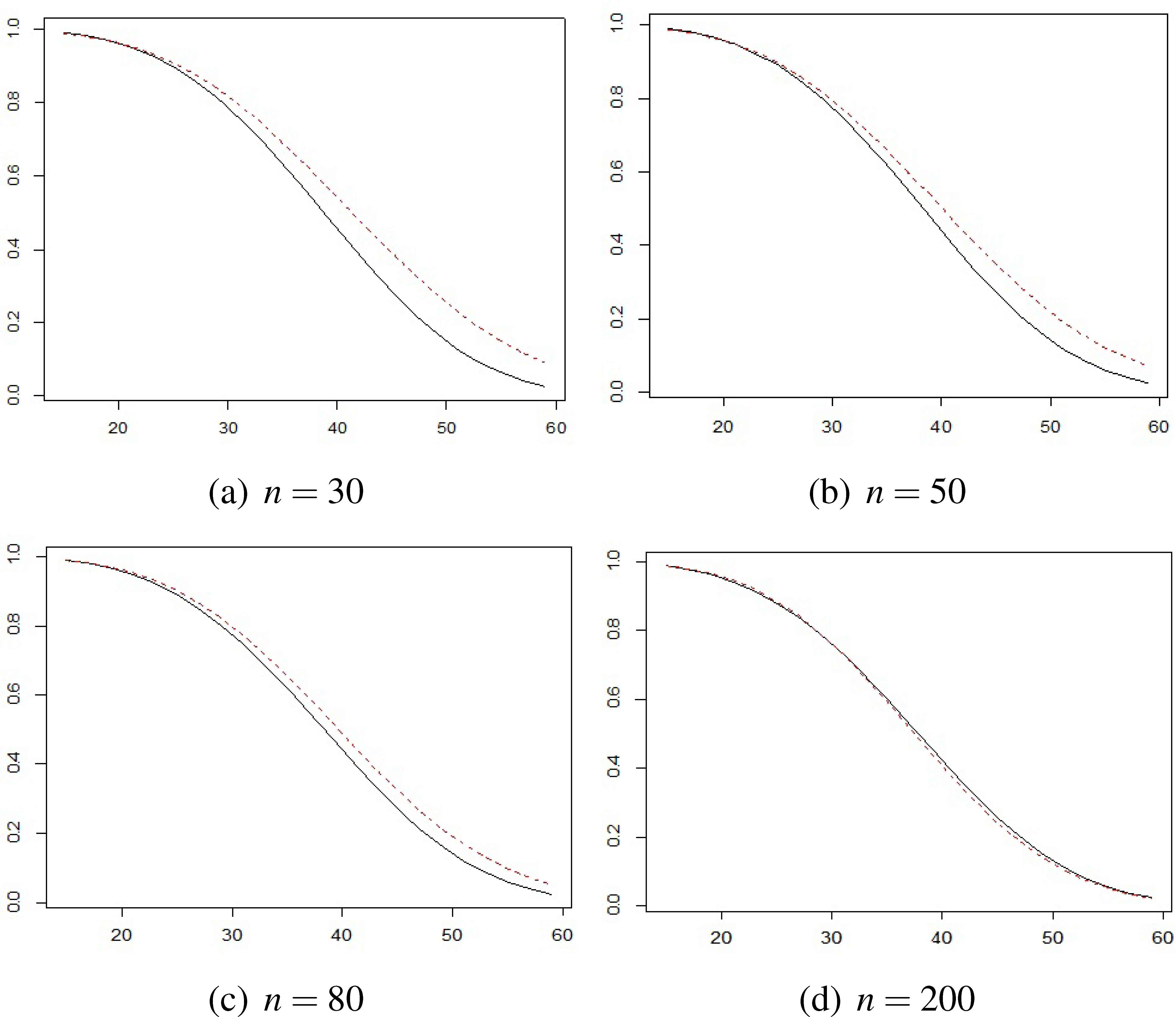
The estimated reliability function in a dependent (solid line) and an independent (dashed line) case under the simple SSADT for simulation data with different sample sizes
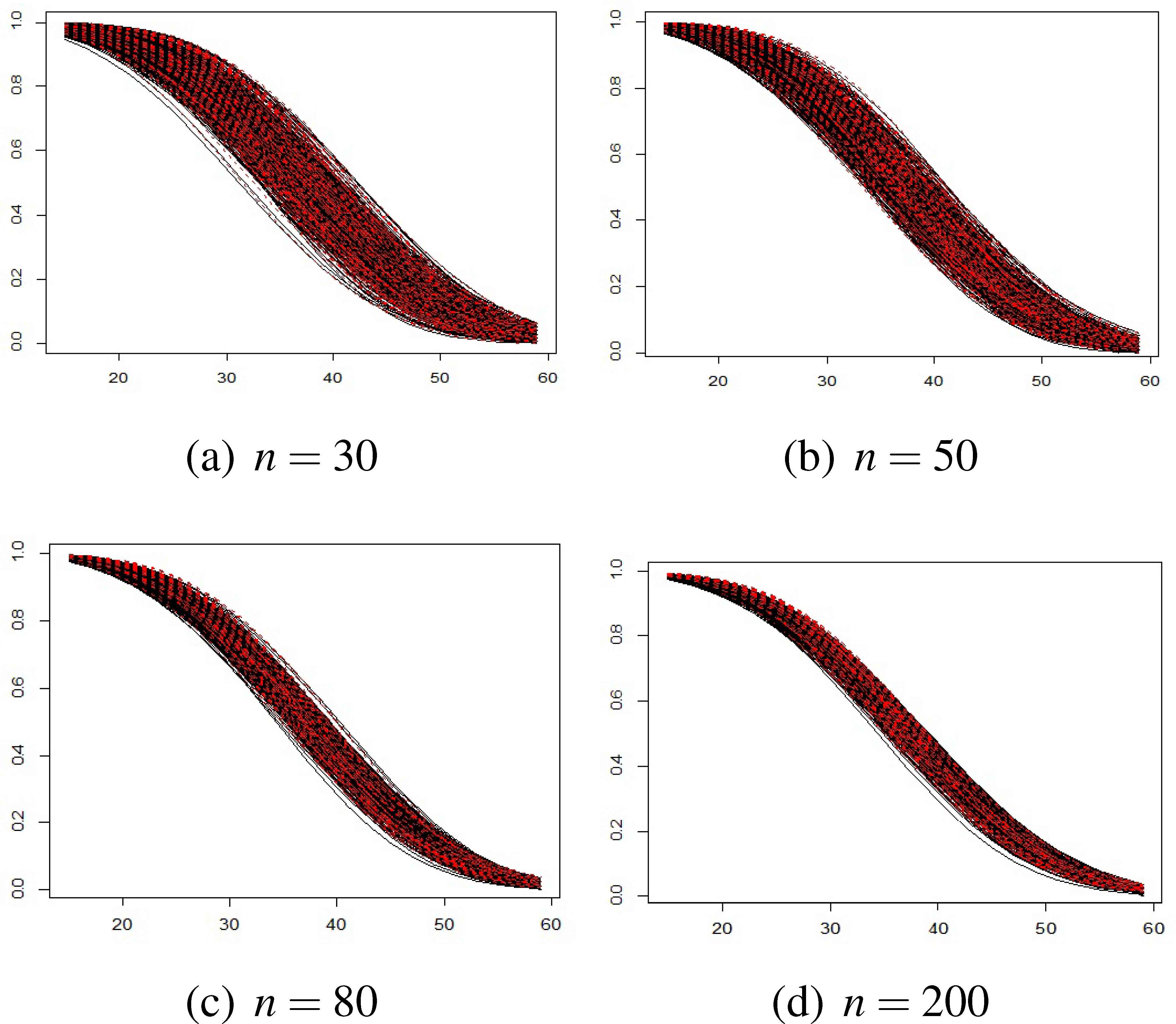
The estimated reliability function in dependent case under the simple SSADT for simulation data with one thousand replications
3.2. Real Data
In this section, we transform two sets of real data into SSADT data by considering a simple step-stress test with a changing time point.
3.2.1. Bus tire data
We use real data collected from 53 bus tires in a normal use environment as presented in a study by [1] who have reported tire wear with two different failure modes: protector zone and side zone. These two failure modes are dependent since the failure rate of both of them depends on degradation.
The method is similar to the previous section with respect to a changing time point of τ1 = 60. According to τ1, 33 out of 53 failure times were at the use stress (S0). As in the previous section, a0j,a1j are the values of A for the j-th unit at the first (normal) and second level of stress, where a1j has been generated from a Weibull distribution with shape parameter, α = 10.60, and scale parameter, β = 4.50. According to the data at normal stress, the estimation of shape and scale parameters are: α = 11.1190, β = 4.4826.Table 3 shows the failure times and corresponding degradation data at each level of stresses.
| S0 | V = 1 | T | 36.8 | 47.3 | 50.8 | 51.0 | 51.2 | 52.1 | 53.0 | 53.8 | 54.3 | 55.0 | 55.2 |
| 56.2 | 56.8 | 56.9 | 57.1 | 57.4 | 57.9 | 58.3 | 58.6 | 59.3 | 59.6 | ||||
| Z(t) | 9.5 | 13.4 | 13.4 | 12.1 | 11.3 | 12.1 | 12.8 | 12.5 | 13.4 | 13.0 | 12.8 | ||
| 13.3 | 13.3 | 13.2 | 12.0 | 12.7 | 10.8 | 12.2 | 12.1 | 13.4 | 13.4 | ||||
| V = 2 | T | 50.0 | 51.0 | 51.7 | 51.7 | 55.0 | 55.0 | 56.0 | 56.6 | 58.1 | 58.9 | 59.0 | |
| 59.2 | |||||||||||||
| Z(t) | 13.3 | 13.1 | 12.5 | 13.2 | 13.1 | 13.2 | 12.5 | 13.2 | 13.2 | 11.7 | 14.0 | ||
| 13.2 | |||||||||||||
| S1 | V = 1 | T | 60.083 | 61.236 | 62.879 | 63.658 | 65.331 | 65.346 | 67.425 | 68.222 | 70.700 | 75.961 | |
| Z(t) | 12.7 | 13.6 | 14.5 | 13.5 | 14.1 | 12.8 | 13.2 | 12.9 | 14.2 | 15.0 | |||
| V = 2 | T | 61.311 | 65.338 | 65.473 | 65.609 | 65.759 | 69.664 | 70.457 | 73.064 | 73.182 | 74.588 | ||
| Z(t) | 13.6 | 13.2 | 13.8 | 13.7 | 13.3 | 13.6 | 13.6 | 15.0 | 15.0 | 15.0 | |||
Time failures and corresponding degradation data at the first and second level of stress for the bus tire data
All model parameters,(α0, β0, θ1, ν1, θ2, ν2, θ), have been estimated using a numerical solution of the likelihood functions (2.14) and (2.15) and reported in Table 4. The last column of Table 4 is the estimated median of the lifetime
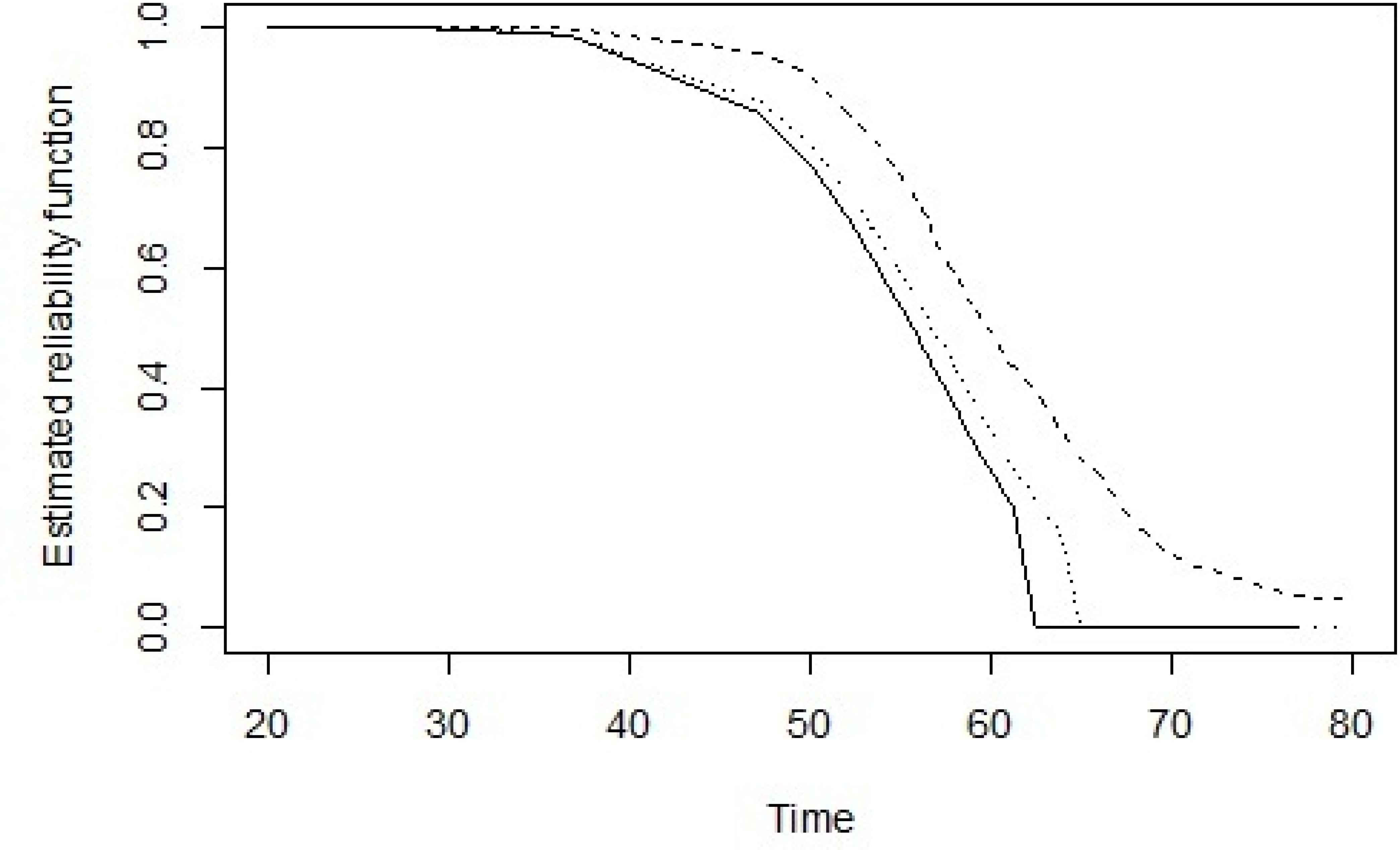
Nonparametric (dashed line) and parametric estimated reliability function in a dependent (solid line) and an independent (dotted line) case under the simple SSADT for bus tire data
| α0 | β0 | θ1 | ν1 | θ2 | ν2 | θ | M | |
|---|---|---|---|---|---|---|---|---|
| Dependent case | 11.119 | 4.4826 | 0.0655 | 12.168 | 0.0663 | 13.046 | 20.22 | 55.88 |
| Independent case | 11.119 | 4.4826 | 0.0616 | 11.611 | 0.0647 | 17.269 | – | 56.79 |
The estimation of parameters with and without dependency for the bus tire data
3.2.2. AMOLED data
In the second example, the real data was collected from plastic substrate active matrix organic light emitting diode (AMOLED). AMOLED is an attractive light device compared to other display devices. In order to achieve SSADT data, the luminance degradation is accelerated using temperature. In this set of data, two failure modes (the organic layer peel-off from the substrate and delamination) expedited by temperature could be observed. We have assumed that the two failure modes are dependent. In the AMOLED data we have 20 failure times with corresponding degradation and different failure modes. The data are reported in [11] and shown in Table 5. The simulated failure times in the second level stress are obtained with a changing time point of τ1 = 1800 [13 failure times are in normal stress level (below 1800)] and the failure rate of each failure time depended on degradation data similar to the previous example.
| S0 | V = 1 | T | 1294.4 | 1462.4 | 1593.6 | 1713.4 | |||||
| Z(t) | 90.42 | 97.37 | 88.49 | 95.18 | |||||||
| V = 2 | T | 1565.8 | 1414.9 | 1592.7 | 1141.4 | 1514.4 | 1505.0 | 1509.6 | 1517.3 | 1267.1 | |
| Z(t) | 97.30 | 93.08 | 90.82 | 97.80 | 97.42 | 96.02 | 93.28 | 90.24 | 98.43 | ||
| S1 | V = 1 | T | 2074.708 | 2400.158 | 1884.541 | 1883.251 | 1978.770 | 1872.205 | |||
| Z(t) | 90.20 | 87.37 | 84.46 | 85.27 | 76.87 | 91.69 | |||||
| V = 2 | T | 1824.737 | |||||||||
| Z(t) | 97.067 | ||||||||||
Failures and corresponding degradation data at the first and second level of stress for the AMOLED data
A Weibull distribution with shape and scale parameters α = 10.749, β = 16.381 was fit to a0j, j = 1,…,13. The a1j were also generated according to a Weibull distribution with shape parameter 2.79 and scale parameter 10. The estimate of all parameters (α0, β0, θ1, ν1, θ2, ν2, θ) and the median of the lifetime
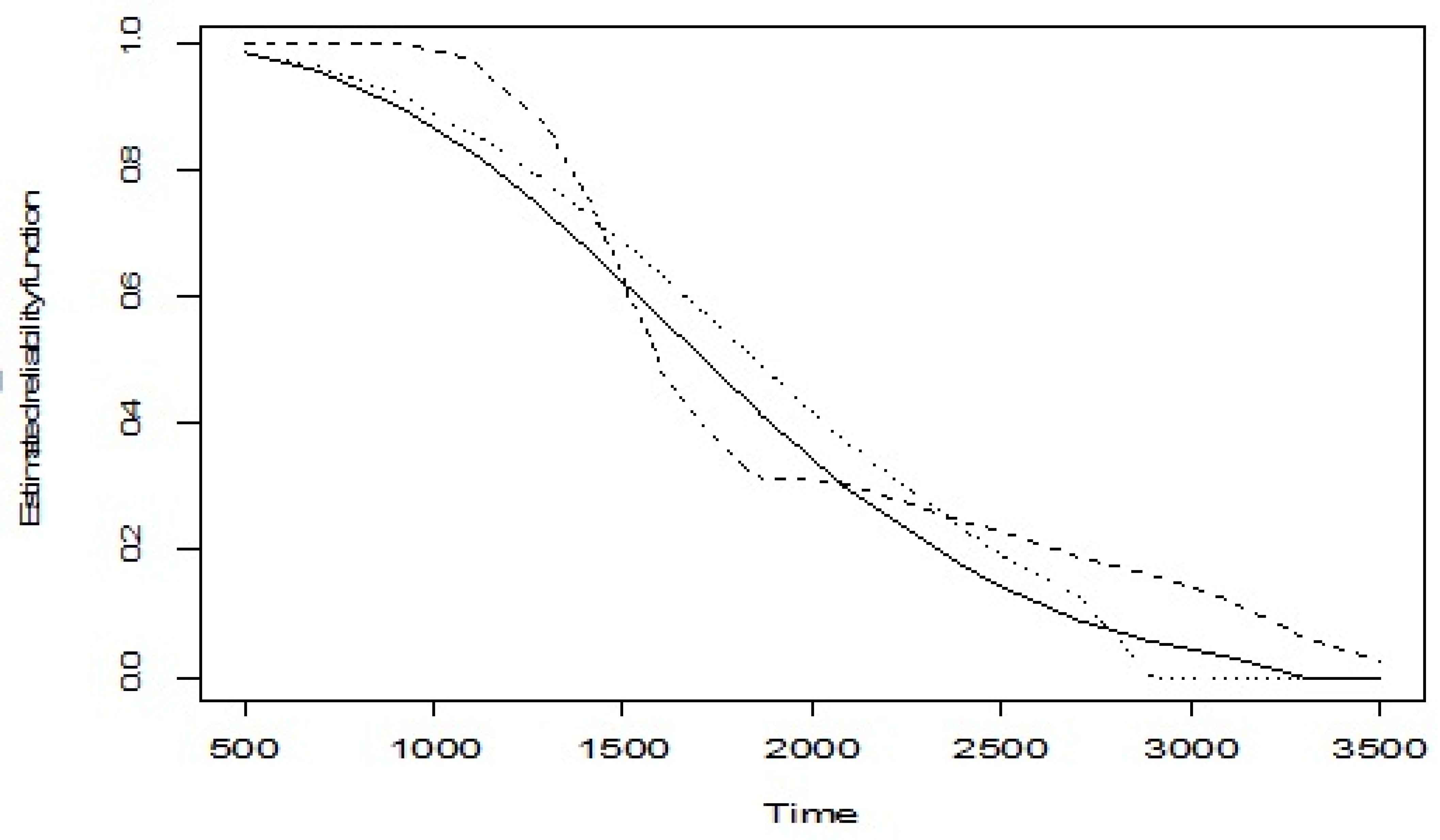
Nonparametric (dashed line) and parametric estimated reliability function in a dependent (solid line) and an independent (dotted line) case under the simple SSADT for AMOLED data
| α0 | β0 | θ1 | ν1 | θ2 | ν2 | θ | M | |
|---|---|---|---|---|---|---|---|---|
| Dependent case | 10.749 | 16.38 | 0.0067 | 11.92 | 0.008 | 20.96 | 27.62 | 1765.95 |
| Independent case | 10.749 | 16.38 | 0.0074 | 14.59 | 0.0096 | 48.70 | – | 1844.03 |
The estimation of parameters with and without dependency
4. Sensitivity analysis
In this section, we performed two sensitivity analyses. The first analysis explored the effects of changing the copula function on parameter estimation. In the second sensitivity analysis, we sought to explore the impact of the change in change-point of the stress on the parameter estimation under a simple SSADT.
4.1. The effect of changing the copula function on parameter estimation
In order to investigate the effect of changing the copula function on parameter estimation, we applied both simulated and real data. Initially, we conducted a simulation study. The data were generated according to the different copulas (Frank, Clayton, and Gumble) following Section 3, Steps 1-4, where: α0 = 5, β0 = 4, θ1 = 0.06, ν1 = 5, θ2 = 0.06, ν2 = 5, θ = 20 and n = 30. Table 7 shows the estimated parameters. We determined that the Frank copula was more appropriate based on the actual value of the parameters, in addition to SE and MRE of the estimators.
| (α0 = 5 , β0 = 4, θ1 = 0.06, ν1 = 5, θ2 = 0.06, ν2 = 5, θ = 20) | ||||
|---|---|---|---|---|
| Copula | Parameter | Estimate | SE | MRE |
| Frank | α0 | 5.1135 | 0.5686 | 0.0962 |
| β0 | 3.9790 | 0.1520 | 0.0299 | |
| θ1 | 0.0602 | 0.0073 | 0.0923 | |
| ν1 | 5.3335 | 1.1876 | 0.1744 | |
| θ2 | 0.0605 | 0.0068 | 0.0870 | |
| ν2 | 5.2527 | 0.9841 | 0.1628 | |
| θ | 17.2259 | 14.0303 | 0.6130 | |
| Clayton | α0 | 5.0971 | 0.8331 | 0.1171 |
| β0 | 3.9793 | 0.1567 | 0.0318 | |
| θ1 | 0.0560 | 0.0084 | 0.1049 | |
| ν1 | 4.7304 | 1.1916 | 0.1917 | |
| θ2 | 0.0555 | 0.0081 | 0.1058 | |
| ν2 | 4.6548 | 1.1062 | 0.1852 | |
| θ | 30.4304 | 44.2251 | 2.1881 | |
| Gumble | α0 | 5.2004 | 0.7574 | 0.1205 |
| β0 | 3.9692 | 0.1555 | 0.0321 | |
| θ1 | 0.0649 | 0.0085 | 0.1290 | |
| ν1 | 6.1629 | 1.6670 | 0.2954 | |
| θ2 | 0.0655 | 0.0103 | 0.1448 | |
| ν2 | 6.2595 | 1.7361 | 0.3278 | |
| θ | 50.313 | 60.86 | 5.4178 | |
The MLEs of the parameters, and the associated SE and MRE for n = 30 in different copula
Additionally, we used real data based on the original bus tire data set to further investigate the effect of changing the copula function on parameter estimation, [1]. The assumption of dependency between failure modes was valid because we supposed that the failure rates of two failure modes depended on the amount of degradation. We fixed the value of τ1 at 62. Then, we generated accelerated failure times to determine the MLE of the parameters by using numerical methods with 2000 replications. Table 8 lists the results. The simulated and real data examples provided evidence that the parameters of ν1, ν2 and θ, were mostly affected by changing the copula function.
| Copula function | α0 | β0 | θ1 | ν1 | θ2 | ν2 | θ | M |
|---|---|---|---|---|---|---|---|---|
| Frank | 11.5890 | 4.5013 | 0.0637 | 11.6177 | 0.0657 | 13.5076 | 30.1010 | 56.886 |
| Clayton | 11.5890 | 4.5013 | 0.0647 | 13.0798 | 0.0644 | 13.3472 | 89.1893 | 57.1095 |
| Gumble | 11.5891 | 4.5013 | 0.0678 | 16.6345 | 0.0656 | 13.7697 | 25.1193 | 57.4576 |
The estimation of parameters using different copula function
4.2. The effect of the change-point of the stress on parameter estimation
In this section, we investigate the effect of the change-point of the stress on parameter estimation based on the original data set of bus tire data, [1]. Like the previous section, we generate accelerated failure times and estimate the parameters of likelihood function using numerical methods with 2000 replications. These steps are repeated for different values of τ1. The results are shown in Table 9. It is observed that, the change-point of stress has little effect on the estimates of (θ1, ν1, θ2, ν2, θ) , but the effect on the estimates of (α0, β0,M) is significant.
| τθ | 58 | 60 | 62 | 64 | 66 | 68 | 70 |
|---|---|---|---|---|---|---|---|
| n01 | 17 | 21 | 23 | 24 | 26 | 27 | 28 |
| n02 | 8 | 12 | 13 | 13 | 14 | 15 | 18 |
| n11 | 14 | 10 | 8 | 7 | 5 | 4 | 3 |
| n12 | 14 | 10 | 9 | 9 | 8 | 7 | 4 |
|
|
10.3883 | 11.1190 | 11.5890 | 11.6889 | 11.9279 | 11.5398 | 11.1419 |
|
|
4.3935 | 4.4826 | 4.5013 | 4.4992 | 4.5237 | 4.5826 | 4.6611 |
|
|
0.06365 | 0.06361 | 0.06368 | 0.06371 | 0.06375 | 0.06357 | 0.06352 |
|
|
11.5847 | 11.5581 | 11.6177 | 11.6647 | 11.7882 | 11.6169 | 11.5299 |
|
|
0.06564 | 0.0656 | 0.06570 | 0.06572 | 0.06541 | 0.06581 | 0.06571 |
|
|
13.4500 | 13.4081 | 13.5076 | 13.5613 | 13.3389 | 13.7345 | 13.5154 |
|
|
30.6017 | 30.4961 | 30.1010 | 30.1349 | 31.42179 | 30.3591 | 32.8662 |
|
|
55.369 | 56.555 | 56.886 | 56.9045 | 57.3392 | 57.9129 | 58.6766 |
The effect of changing point on the estimation precision with 2000 replications
5. Conclusion and further work
SSADT is one of the most commonly used methods for reducing the required sample size. When we have multiple failure modes in SSADT, it is important to take into account the dependency between them. This article has proposed a modeling approach for simultaneously analyzing dependent failure modes and degradation data under the SSADT. According to this method, we can estimate the reliability function in a dependent case and compare the differences between the dependent and independent cases. This difference is significant in dependent failure modes. Sensitivity analysis also shows that changing the copula function and change-point of the stress affects on a small number of parameters.
In this article, we have assumed that the degradation is linear; failure rates depend on degradation and do not make any assumption about the failure-time distribution. For further analysis, we can change these assumptions. For example, we can consider nonlinear degradation or other forms of failure rates, such as: λk(z(t)) = γk + (θkz(t))νk.
References
Cite this article
TY  - JOUR
AU  - Somayeh Mireh
AU  - Ahmad Khodadadi
AU  - Firoozeh Haghighi
PY  - 2018
DA  - 2018/06/30
TI  - Joint Modeling of Linear Degradation and Multiple Dependent Competing Risks Data under a Step-Stress Accelerated Degradation Test
JO  - Journal of Statistical Theory and Applications
SP  - 340
EP  - 358
VL  - 17
IS  - 2
SN  - 2214-1766
UR  - https://doi.org/10.2991/jsta.2018.17.2.12
DO  - 10.2991/jsta.2018.17.2.12
ID  - Mireh2018
ER  -