
Shannon Information in K-records for Pareto-type Distributions
- DOI
- 10.2991/jsta.2018.17.3.3How to use a DOI?
- Keywords
- K-record values; K-record times; Shannon information; Digamma function; Zeta function; Differential entropy; Record data
- Abstract
Pareto distributions provides models for many applications in the social, natural and physical sciences. In this paper, we derive the Shannon information contained in upper (lower) k-record values and associated k-record times of Pareto-type distributions for a finite sample of fixed size and for an inverse sampling plan. Properties of the Shannon information of the k-record values associated with Pareto-type distributions are investigated, both analytically and numerically.
- Copyright
- © 2018, the Authors. Published by Atlantis Press.
- Open Access
- This is an open access article under the CC BY-NC license (http://creativecommons.org/licences/by-nc/4.0/).
1. Introduction
The origin of the term entropy goes back to the works of Clausius (1864) and Boltzmann (1872) in thermodynamics. The idea of information-theoretic entropy was first introduced by Shannon (1948). Park (1995), Ebrahimi et al. 2004 and Oluyede (2006) obtained various results on the information properties of order statistics. Yari and Borzadaran (2010) calculated the Shannon entropy for Paretotype distributions and their order statistics. Baratpour et al. 2007 derived some results related to the Shannon entropy and Rényi entropy for record values.
In 1976, Dzubdziela and Kopociński introduced the concept of k-records which were further studied by Grudzieén and Szynal (1985), Raqab and Amin (1997) and called Type 2 k-records by Arnold et al. 1998. For k = 1, the usual records are obtained.
Madadi and Tata (2011) presented results on the Shannon information contained in upper (lower) record values and associated record times in a sequence of independent identically distributed continuous random variables. They also considered the Shannon information contained in record data from an inverse sampling plan. In 2014, they generalized these results to k-records. Afhami and Madadi (2013) derived the exact analytical expressions for the Shannon entropy of generalized order statistics from the Pareto (IV) distribution and related distributions.
In this paper, we obtain the Shannon information contained in upper (lower) k-record values and k-record times of a random sample of size n (n ≥ k) and of an inverse sampling plan for Pareto-type distributions. The paper is organized as follows: In Section 2, we present some preliminary results. Section 3 contains the main results of the paper. In this section, we derive the Shannon information contained in the data consisting of all upper and lower k-record values and associated k-record times of a random sample of size n and of an inverse sampling plan for Pareto-type distributions. We also present some results of the differential entropy for a finite sample of fixed size and for an inverse sampling plan. Finally, Section 4 contains a conclusion.
2. Preliminaries
In this section, we review some basic notations and definitions concerning Pareto-type distributions, k-records and entropy which will be needed in the next section.
2.1. Pareto-type distributions
A general version of Pareto-type distributions, called the Pareto (IV) distribution, is discussed in chapter 3 of Arnold (1983). The cumulative distribution function of this family is
- •
- •
The Burr (XII) distribution is a special case of the Pareto (IV) distribution in which µ = 0,
andwhere α > 0. We denote this distribution by Pareto (α) and note that Zα has the same distribution as
2.2. Shannon information
Consider a discrete random variable X such that P{X = xi} = pi, i = 1,2,··· and
Lemma 2.1.
If X = θZγ + µ, then
So,
The Shannon entropy of the random variable X is a mathematical measure of information which measures the average reduction of uncertainty of X. Because of its descriptive character, analytical expressions for univariate distributions have been obtained, among others, by Cover and Thomas (2006).
2.3. k-record data
Let {Xn : n = 1,2,…} be a sequence of independent and identically distributed (i.i.d) random variables with absolutely continuous cumulative distribution function F(x; θ) and probability density function f(x; θ). We are interested in the Shannon information (SI) contained in the sequence of k-records. A k-record is basically the k-th largest observation in a partial sample. More precisely, let Xi:n denote the i-th order statistic from a random sample of size n. We define upper k-record times Tn,k and upper k-record values Rn,k as follows :
- (i)
T1,k = k and R1,k = X1:k,
- (ii)
Tn,k = min{j : j > Tn−1,k, Xj > XTn−1,k−k+1:Tn−1,k} and Rn,k = XTn,k − k + 1 : Tn,k, (n ≥ 2).
Suppose Nn,k be the number of k-record values in X1,…,Xn. Lower k-record values, lower k-record times and the number of lower k-records are similarly defined (Arnold et al., 1998).
In the case of record and k-record data from a random sample of size n, Madadi and Tata (2011, 2014) obtained the SI contained in the last record (maximum), upper k-record values with associated k-record times, denoted by
In an inverse sampling plan (ISP), one takes observations until a fixed number m of k-records is reached. Denote the SI contained in all upper k-record values, the last upper k-record and all upper k-record values together with associated k-record times by
Madadi and Tata (2011) showed that the SI contained in the last upper record is
Madadi and Tata (2014) also proved that the SI contained in the data consisting of all upper k-record values and k-record times of a random sample of size n (n ≥ k) is given by
They also showed that the SI contained in all of k-record values, last upper k-record and all of upper k-record values and times of an ISP are respectively obtained as
Note that for k = 1, i.e. for ordinary records,
3. Shannon information in k-records for Pareto-type distributions
In this section, we compute the SI in k-records of Pareto-type distributions for a finite sample of fixed size as well as for an inverse sampling plan.
3.1. Shannon information in a finite sample
Since the number of observations n is fixed (and the number of records is random), the last upper record is the maximum in the sample. From (2.5) and (2.6) , we have
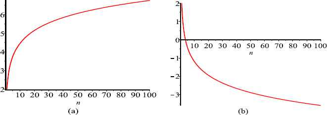
(a) and (b) represent
One can easily see that
- (i)
- (ii)
- (iii)
- (iv)
For each fixed n,
- (v)
Theorem 3.1.
For Pareto (1), the SI contained in all the upper and lower k-record values together with k-record times of a random sample of size n (n ≥ k) are equal to
Also for k = 1, we obtain
Corollary 3.1.
For
Corollary 3.2.
The SI contained in all k-record values and k-record times of a random sample of size n (n ≥ k) from the Pareto (IV) distribution are
For ordinary records, these information can be written as
- (i)
- (ii)
- (iii)
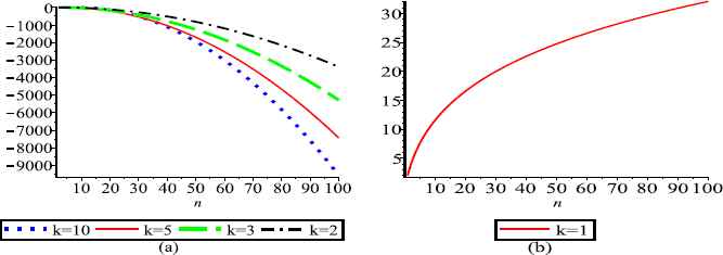
(a) and (b) represent
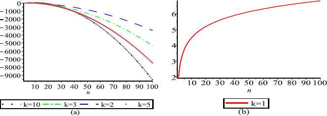
(a) and (b) represent
3.2. Shannon information in an inverse sampling plan
In an inverse sampling plan, we take observations until a fixed number m of k-records is reached. Here, we compute the SI of k-records for an inverse sampling plan from Pareto-type distributions and discuss their properties.
Theorem 3.2.
The SI contained in the m-th upper and m-th lower k-record values from Z1 are given by
Remark 3.1.
For m = 1, we have
Corollary 3.3.
For Zα, we obtain
Corollary 3.4.
The SI contained in the m-th upper and m-th lower k-record values from the Pareto (IV) are
Let
- (i)
- (ii)
for each fixed k,
- (iii)
- (iv)
- (i)
- (ii)
- (iii)
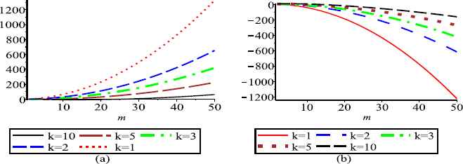
Fig. 4. displays a graphical representation of
Let
- (i)
- (ii)
- (iii)
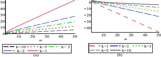
(a) and (b) represent
Remark 3.2.
For m = 1, we have
- (i)
- (ii)
Theorem 3.3.
The SI contained in all of the first m upper and m lower k-record values of an ISP are respectively given by
Corollary 3.5.
For Pareto (I) with parameter α, we have
Corollary 3.6.
For the Pareto (IV), one can obtains
- (i)
- (ii)
- (iii)
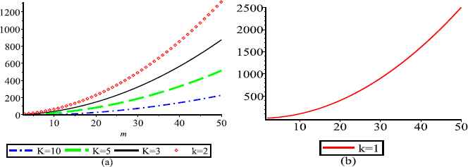
(a) and (b) represent
Remark 3.3.
Note that for k = 1, i.e. for ordinary records, it is easy to see that the differential entropy has the following properties
- (i)
- (ii)
The sequence
- (iii)
- (iv)
- (v)
∀m ≥ 7,
- (i)
- (ii)
Theorem 3.4.
The SI contained respectively in the upper and lower k-record values and associated k-record times for k > 1 are obtained as
Remark 3.4.
Note that for k = 1, (3.13) and (3.14) lead to
Corollary 3.7.
For Zα, we have
Corollary 3.8.
For the Pareto (IV), we have
- (i)
- (ii)
For each m ≥ 8, we have
(a) and (b) represent
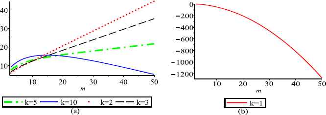
(a) and (b) represent
4. Conclusions
In this paper, we obtained the Shannon information in k-record in a sample of fixed size as well as in an inverse sampling plan for Pareto-type distributions. Properties of entropies for k-record values for Pareto-type distributions are also investigated.
Acknowledgments
The authors are grateful to the editorial board of Journal of Statistical Theory and Applications (JSTA), in particular, Professor Hamedani and would like to thank two anonymous referees for useful comments and suggestions that lead to this improved version of the paper.
References
Cite this article
TY  - JOUR
AU  - Zohreh Zamani
AU  - Mohsen Madadi
PY  - 2018
DA  - 2018/09/30
TI  - Shannon Information in K-records for Pareto-type Distributions
JO  - Journal of Statistical Theory and Applications
SP  - 419
EP  - 438
VL  - 17
IS  - 3
SN  - 2214-1766
UR  - https://doi.org/10.2991/jsta.2018.17.3.3
DO  - 10.2991/jsta.2018.17.3.3
ID  - Zamani2018
ER  -