Definition 1.1.

The characteristic function of a stable random variable, say X, has the form

where sgn(.) is the well-known sign function.

Definition 1.2.

Let Y be a d-dimensional sub-Gaussian α-stable (sub-Gaussian SαS) random vector. Then, the characteristic function of Y can be written as

where Σ is a d × d positive definite matrix and μ ∈ IR^d is the location parameter.

2.1. EM algorithm and extension

Missing or incomplete observations frequently occurs in the statistical literature. The EM algorithm, introduced in [7], is a popular inferential tool for such a situation. The application of the EM algorithm also includes cases with latent variables or models with random parameter provided that they are formulated as a missing value problem. For a brief description of EM methodology, let x = (x₁,…, x_n) denote the complete observations follow the density function f(x|θ). We denote x = (y, z), where z denotes missing samples and y accounts for the available observations, [16]. The computation and maximization of

are difficult in such a case. So, we propose to use the EM algorithm. Let L_c(θ) = f((y, z)|θ) be the complete data likelihood function. The EM algorithm works by maximization of the conditional expectation of the complete log-likelihood function Q(θ|θ^(t)) = E(l_c(θ; x)|y,θ^(t)) given the available data and a current estimate θ^(t) of the parameter (here, l_c(θ; x) indicates on the logarithm of L_c(θ)). Since missing values are unobservable, we replace them by their expectation, given observed values and a current guess (or estimate) for θ. Each iteration of the EM algorithm involves two steps as:

1. 1.

   Expectation (E) step: Compute Q(θ|θ^(t)) at t-th iteration.

2. 2.

   Maximization (M) step: Maximize Q(θ|θ^(t)) with respect to θ to get θ^(t+1).

The E and M steps, in above, are repeated until convergence occurs. When the M step of the EM algorithm becomes analytically intractable, we follow the idea of implying this step using a sequence of conditional maximization, known as the CM step. The resulting procedure is known as the ECM algorithm, [18]. A faster extension of the EM algorithm is the so-called ECME algorithm introduced in [14]. It should be noted that all the EM, ECM and ECME have the same E step. The ECME algorithm works by maximizing the constrained Q(θ|θ^(t)) via some CM steps and maximizing the constrained marginal likelihood function, [1]. Sometimes implementation of the EM algorithm is difficult. In this situation, another extension of this algorithm, called the stochastic EM (SEM) is useful, [2], [3], and [4]. Each SEM works by simulating missing data from conditional density f(z_i|θ^(t), y_i); for i = 1,…, n and replacing it into the complete likelihood function. Then, we apply the EM algorithm for the pseudo-complete sample where (Z1(t),…,Zn(t)) are simulated ones. The updated parameter is then used to simulate from f(z_i|θ^(t+1), y_i); for i = 1,…, n. This process is repeated until convergence occurs for the distribution of the {θ^(t+1)}. Under some mild regularity conditions, {θ^(t+1)} constitutes a Markov chain that converges to a stationary distribution, [11]. The number of iterations is determined via an exploratory data analysis approach such as a graphical display. Another example presented in [11] is to consider a total of 300 iterations of the SEM for estimating the parameter of modulus of rupture of 50 observations of fir woods after fitting a two-parameter Weibull model under Type-I censored scheme (the data were censored at 1.6 which corresponds to a censoring of rate 34%). As pointed out by the authors, the SEM is generally very robust to the starting values. Using a burn-in of M₀ iterations, the sequence {θ^(t)} is expected to be close to some stationary point. After a sufficiently large number of iterations, say M, the SEM estimation of θ is given by

where M₀ is burn-in size. Summarizing the above statements, each iteration of the SEM algorithm consists of two steps as follows.

1. 1.

   Stochastic imputation (S) step: Impute the simulated missing values and constituting the pseudo-complete log-likelihood function at t-th iteration.

2. 2.

   Maximization (M) step: Find a θ, say θ^(t+1), which maximizes the pseudo-complete log-likelihood function at t-th iteration.

The S and M steps, in above, are repeated until convergence occurs.

2.2. Properties of symmetric and positive stable laws

Suppose that Y₁ and Y₂ > 0 are independent stable random variables, Y₁ ~ S(α₁, 0, σ, 0) and Y₂ ~ S(α₂, 1, (cos(πα₂/2))^1/α₂, 0) for 0 < α₂ < 1. Then, Y1Y21/α1∼S(α1α2,0,σ,0) , known as the product property in the literature. Based on product property, one can write

where Y ~ S(α, 0, σ, μ), P ~ S(α/2, 1, (cos(πα/4))^2/α, 0), and N₁ is a zero-mean Gaussian random variable with variance 2σ². So, where N₂ is a Gaussian random variable with mean μ and variance 2pσ². As the second useful property, assume that P ~ S(α/2, 1, (cos(πα/4))^2/α, 0). Then, where E is an exponential random variable with mean one and W(ν) is a Weibull random variable, independent of E, with density function f_W (w) = νw^ν−1 exp {−w^ν}; for w > 0. Since 0 < α/2 < 1 and β = 1, then P sometimes is called the positive stable random variable. For a proof of (2.4), we refer readers to [17] and [30, p. 15].

3.1. The first approach

Let y = (y₁,…, y_n) be a random sample from a SαS distribution. Refer to (2.3) and consider p = (p₁,…, p_n) as the vector of missing observations. The complete data likelihood L_c(Θ) is factored into the product of the marginal densities of P_i and the conditional densities of Y_i given P_i. So, the complete data log-likelihood can be written as

where Θ = (θ^T, α)^T, θ = (μ, σ)^T. It follows that and where C is a constant independent of the parameter θ and f_P(.) denotes the density function of the positive stable random variable P. Conditional expectation of the complete data log-likelihood Q(Θ|Θ^(t)) = E(l_c(Θ; p)|y, Θ^(t)) is given by where ei(t,s)=E(P-1|yi,μ(t),σ(s),α(s)) , Θ^(t) = (θ^(t)T, α^(t))^T and θ^(t) = (μ^(t), σ^(t))^T. Here, ei(t,s) is the posterior mean of 1/P given y_i and Θ^(t); for i = 1,…,n. Thus, the EM algorithm’s steps are

• •

  E step: Given current estimation of Θ, Θ^(t), compute ei(t,t) .

• •

  CM step: Update θ^(t) as θ^(t+1) by maximizing Q(Θ|Θ^(t)) with respect to θ to obtain

  (3.1)μ(t+1)=∑i=1nyiei(t,t)∑i=1nei(t,t),

  (3.2)σ(t+1)=∑i=1n(yi-μ(t+1)2ei(t+1,t))2n.

• •

  CML step: Update value of α^(t) by maximizing the marginal log-likelihood function as

  α(t+1)=argmaxα∑i=1nlogfY(yi|μ(t+1),σ(t+1),α),

  where f_Y(.) is the SαS density function. Under the methodology that we follow here, the CML step itself contains an SEM algorithm (This is because the density function of SαS random variable has no closed-form expression). In the following, two steps of the SEM are described.

• •

  The first step of CML: Let E₁, E₂,…, E_n be independent exponentially distributed random variables with mean one. At (t + 1)-th iteration, assume that μ^(t+1) and σ^(t+1) are known. Let Y^′_i = (Y_i − μ^(t+1))/σ^(t+1) and Yi″=Yi′/Ei ; for i = 1,…,n. Then it follows, from (2.2) and (2.4), that

  Yi″|Wi=wi~N(0,2wi2),Wi~W(α).

  Considering w₁,…, w_n as missing observations, the complete data likelihood L_c(Θ) is factored into the product of the marginal densities of W_i and the conditional densities of Y″_i given W_i. So, the complete data log-likelihood can be written as

  (3.3)lc(α)=C+nlogα+(α-1)∑i=1nlogwi-∑i=1nwiα.

• •

  The second step of CML: Simulate the vector w = (w₁,…, w_n) from conditional distribution of W_i given y″_i; for i = 1,…,n, and Θ^(t) using the Monte Carlo method at the m-th cycle of the S step of the SEM.

• •

  The third step of CML: Substitute w in (3.3) and maximize it with respect to α to find α^(t+1). Then, repeat the algorithm from E step for M times to obtain Θ^(t) as

  Θ^=1M-M0∑t=M0+1MΘ(t),

  where M₀ is burn-in size. Maximizing (3.3) with respect to α in each cycle is equal to computing the ML estimation of a Weibull distribution with shape parameter α.

3.2. Computational considerations of the first approach

In the E step of the algorithm, we need to calculate the conditional mean ei(t,t) and ei(t+1,t) in iteration steps (3.1) and (3.2), respectively. Unfortunately, this quantity cannot be calculated analytically. At (t + 1)-th iteration of the E step, we have

and after obtaining μ^(t+1) in the CM step, by replacing μ^(t+1) in (3.4) we obtain ei(t+1,t) . Then, we update σ^(t+1) in the CM step. Direct computation of ei(t,t) using numerical integration faces with problem when |y_i|, for i = 1,…,n, is large. To avoid computational issues, we use the series representation for the density function f_P(.|α^(t)) of S(α^(t)/2, 1, (cos(πα^(t)/4))^2/α(t), 0) as for large k, [10] and [25]. Substituting the right-hand side of (3.5) into (3.4), after a suitable change of variable and simplifications, we get where Γ(.) denotes the well-known gamma function. It should be noted that series in numerator and denominator of (3.6) converge for where k is sufficiently large. This makes the computations to be fast. We found that choosing k = [min(168, 168/α^(t))], where [x] denotes the integer part of x, yields an almost exact evaluation of f_P (.|α^(t)) in (3.5) and so of ei(t,t) in (3.6). For those y_i that series in (3.5) does not converge, we use Monte Carlo based approximation of ei(t,t) given by where P_j ~ S(α^(t)/2, 1, (cos(πα^(t)/4))^2/α(t), 0); for j = 1,…, N, is simulated using the method given in [5]. During our simulation, we set N = 2000.

As the CML step itself contains a SEM algorithm, simulation from conditional distribution of W_i given yi″=(yi-μ(t+1))/(σ(t+1)ei) (e_i, here, denotes an observation from standard exponential distribution) and α^(t) can be performed using Metropolis-Hasting algorithm. We follow our simulation based on Weibull distribution with the shape parameter α^(t) as the candidate. The acceptance rate, A_wi, becomes

The main drawback of the Metropolis-Hasting algorithm is that the new values may have little chance for acceptance in each iteration. In our study, the acceptance rate decays when y″_i gets large. Due to the heavy tail property of stable distribution, large values are likely to happen. Therefore, we adopt a rejection sampling in m-th cycle of the SEM algorithm of the CML step to generate from the posterior distribution of W_i given y″_i and α^(t+1); for i = 1,…, n. To describe this scheme, we note that the density function as a part of the conditional (posterior) density function is bounded by some constant independent of w_i. More precisely Hence, a rejection sampling is employed to generate from the posterior distribution by the following steps.

1. 1.

   Simulate a sample from a Weibull distribution, say w_i, with shape parameter α^(t+1)and scale unity.

2. 2.

   Generate a sample from a uniform distribution U(0,exp{-0.5}/(2π|yi″|)) , say u.

3. 3.

   If u<wi4πexp{-yi″2wi24} , then accept w_i as a generation from f_Wi|Y″i(w_i|y″); otherwise, go to 1.

While we expect that the rejection sampling works satisfactorily, it faces with the problem when |y″_i| is so large. In this case that the machine sets the quantity wi4πexp{-yi″2wi24} to zero and consequently generation from posterior density is so time consuming, we use the mode of the posterior density as a generation from the posterior distribution. It is not hard to check that the mode of the posterior distribution W_i|Y^″_i = y^″_i is obtained as a solution of the equation

Our studies reveal that if |y″_i| is so large that machine sets the quantity wi4πexp{-yi″2wi24} to zero, then choosing the mode of posterior distribution described by (3.7), as an observation from this distribution not only improves the accuracy of the simulation, but also accelerates the EM algorithm implementation.

3.3. The second approach

The first approach works efficiently, but it can be improved to reduce computational complexity by relaxing some CM steps for computing μ^(t+1) and σ^(t+1). This approach significantly reduces the processing times for implementing the EM algorithm. In the CM step of the second approach, we only update μ while both σ and α are updated through the SEM in the CML step. Like the previous approach, the location parameter is updated through (3.1). Let E₁, E₂,…, E_n be independent exponentially distributed random variables with mean one. At (t + 1)-th iteration of the first step of the CML, assume that μ^(t+1) is known. Let Y^′_i = (Y_i − μ^(t+1)) and Yi″=Yi′/Ei ; for i = 1,…, n. It follows that

The complete data log-likelihood can be written as By maximizing (3.8) with respect to σ and α, we find and α^(t+1) is the solution of where w_i is simulated from conditional distribution of W_i given y″_i and Θ^(t); for i = 1,…,n, using rejection sampling at the m-th cycle of the SEM step. Once σ^(t) and α^(t) are updated, we implement the E step and repeat the algorithm for a number of M times and obtain Θ^ as In the first approach, we need to compute ei(t,t) for updating μ^(t) and ei(t+1,t) for updating σ^(t); for i = 1,…,n. But in the second approach, the sequence of ei(t,t) updates μ^(t) and σ^(t) will be updated in the second step of the CML. This yields a considerable reduction in implementing time of the EM algorithm compared with the first approach.

Corollary 4.1.

The updated dispersion matrix Σ^(t+1) in (4.4) is positive definite.

4.1. Computational considerations

At (t + 1)-th iteration, updating μ^(t) in (4.2) needs computing ei(t,t) . For this, when Di(t)=(yi-μ(t))T(Σ(t))-1(yi-μ(t)) is large, ei(t,t) is evaluated approximately as

where and k = [min(168, 168/α^(t))] in (4.6). If Di(t) does not lie in (4.7), we use the Monte Carlo based approximation of ei(t,t) as where Λ_j ~ S(α^(t)/2, 1, (cos(πα^(t)/4))^2/α(t), 0) for large N. As before, we set N = 2000 for implementing the EM algorithm. To construct the pseudo-complete data, w_is are generated in (4.3) through a rejection sampling by the following steps.

1. 1.

   Simulate a sample from a Weibull distribution, say w_i, with shape parameter α^(t+1) and scale unity.

2. 2.

   Define b=dd/2((yi″)TΣ-1yi″)-d/2exp{-d/2}(2π)d/2|Σ|1/2 and generate samples from a uniform distribution U (0, b), say u.

3. 3.

   If u<widexp{-12((yi″)TΣ-1yi″)wi2}(2π)d/2|Σ|1/2 , then accept w_i as a generation from fWi|Yi″(wi|yi″) ; otherwise, go to 1.

if (y″_i)^T ∑⁻¹y″_i is so large, we impute wi=d((yi″)TΣ-1yi″)-1/2 .

5.1. Simulation study in univariate case

We compare the performance of the ML, SQ, CF, and the EM methods for estimating the parameters of SαS distribution through simulation. Comparisons are based on square root of the mean-squared error (RMSE) criterion. In the simulation, the RMSE was computed for sample sizes of n = 200, 500, and 1000. The number of replications is N = 1000. The parameters were selected as: μ = 0, σ = 0 5, 1, 2, and α = 0.4, 0.6, 0.8, 0.9, 1.1, 1.2, 1.4, 1.6, 1.8, 1.9. The plots of the computed RMSE for all estimators are shown in Figures 1–3 . It should be noted that the estimation results for the evaluated ML approach (Nolan’s Method [21]) are not reliable for α < 0.4 and so are not shown in the Figures 1–3. The smoothed version of the actual values plotted in these figures is obtained using the lowess package (see [6]) with the following settings: the smoothing span is considered to be 2/3, the number of iterations is 3, and the speed of computations is determined by 0.01th of the range of the α values.

Fig. 1.

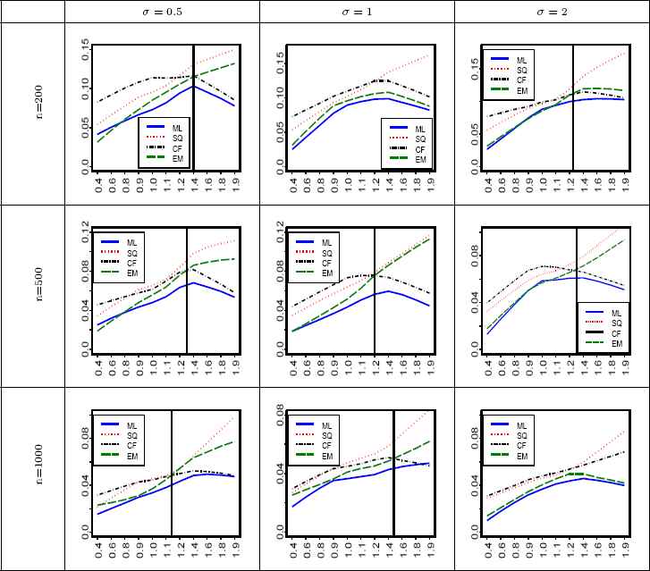
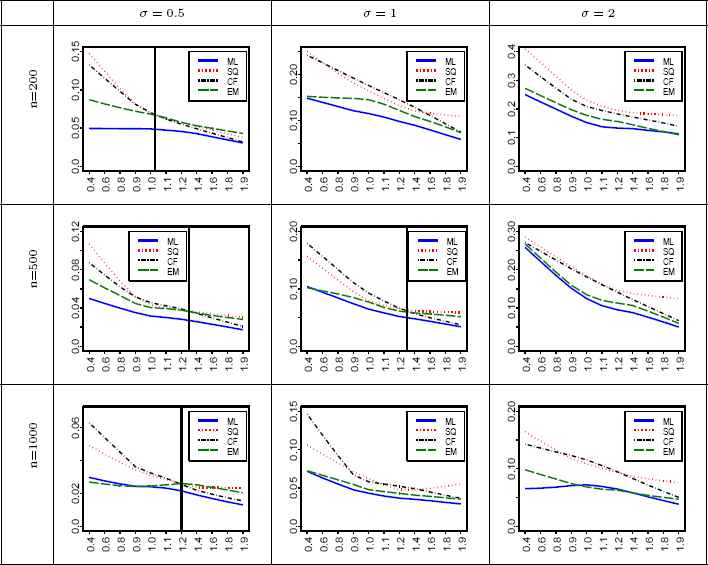
RMSE of α^ for different values of σ = 0.5, 1, 2 and for 0.4 ≤ α ≤ 1.9. In all sub-figures x-axis is values of α and y-axis is RMSE of α^ .

Fig. 2.

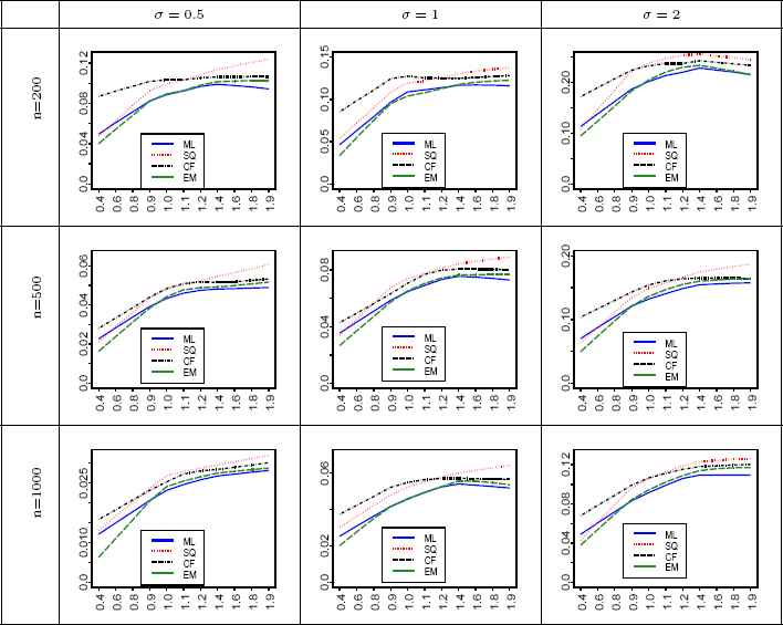
RMSE of σ^ for different values of σ = 0.5, 1, 2 and for 0.4 ≤ α ≤ 1.9. In all sub-figures x-axis is values of α and y-axis is RMSE of σ^ .

Fig. 3.

RMSE of μ^ for different values of σ = 0.5, 1, 2 and for 0.4 ≤ α ≤ 1.9. In all sub-figures x-axis is values of α and y-axis is RMSE of μ^ .

In each sub-figure of Figures 1 - 3, the vertical line indicates that the proposed EM algorithm works better than the CF and SQ methods for those α lie in the left side of the line. When the EM algorithm always works better, such a line is not shown. By considering the location parameter as zero, the following results are obtained from simulation and show how RMSE of the estimators varies in terms of σ, α and n:

1. 1.

   EM-based α^ and σ^ have better performance than the SQ-based and CF-based α^ and σ^ for α < 1.1 in all cases, where shown in Figures 1 and 2, respectively.

2. 2.

   EM-based μ^ shows better performance than the SQ and CF for all α, ref. Figure 3.

3. 3.

   RMSE of the EM-based α^ and σ^ are smaller than the SQ-based α^ and σ^ .

4. 4.

   We know that the ML method gives the efficient estimation particularly when sample size gets large. But, sometimes the EM-based α^ and σ^ outperform the ML counterparts. This occurs, because STABLE gives the approximated ML estimation, not the exact ML estimation.

5. 5.

   RMSE of all estimators decreases by increasing the sample size n.

Along with the simulation, we investigate the execution time for different sample sizes and scale parameters in the univariate case. The results are given in Table 1. For this, all runs are performed on a machine with 3.5 GHz Core(TM) i7-2700K Intel(R) processor and 8 GB of RAM. It should be noted that implementing of the ML, CF, and SQ approaches, with settings given in Table 1, takes less than 0.5 second.

5.2. Real data analysis in the univariate case

For real data application, we select the Bovespa (São Paulo Stock Exchange), CAC40 (Bourse de Paris) and DAX (German Stock Index) indices from WMI data set. The empirical distributions of these three sets of data show symmetric pattern around the origin whose tails are heavier than the normal model. We apply the ML, CF, SQ, and EM methods to estimate the parameters of the fitted stable distributions. It should be noted that the sample median is used as an initial value for the location parameter to implement the EM algorithm. Initial values for the tail and scale parameters are obtained by applying the method of the logarithmic moment. This approach, for a symmetric stable distribution, estimates the parameters using the first and the second order moments of the logarithm of a zero-location symmetric stable random variable Y, i.e. L₁ = E(log |Y|) and L₂ = E(log |Y| − L₁)², respectively. Assuming that data, after subtracting from the sample median, follow a zero-location symmetric stable distribution, the parameters α and σ are estimated by equating the sample logarithmic moments to the quantities L₁ and L₂, [20] and [32]. Figure 4 displays cycles of the EM algorithm for M = 120 and M₀ = 70.

Fig. 4.

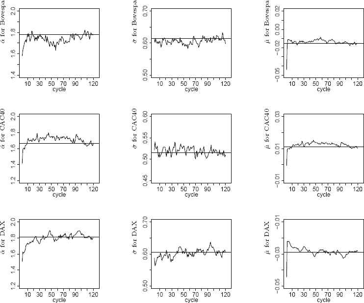
Estimated values of α, σ, and μ with M = 120 cycles each with n = 2535 samples for Bovespa, CAC40 and DAX indices selected from WMI data set.

Estimated parameters, along with the Kolmogorov-Smirnov (K-S) and Anderson-Darling (A-D) test statistics are given in Table 2. More analyses reveal that stable model captures the general shape of the empirical histogram well and the main difference between fitnesses occurs at the origin for the height of peaks. As it is seen, EM algorithm gives satisfactory results.

Fig. 5.

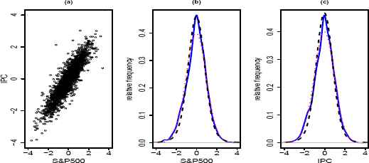
Scatterplot of the IPC index versus S&P500 index (a) shows that distribution of points on a plane is roughly elliptical. Points in scatterplot are a number of n = 2535 daily returns from April 1, 2000 through September 22, 2009. Marginal density plots of the S&P500 (b) and IPC (c) show that the stable distribution (black dashed line) provides a better fit than the normal (red dotted line) distribution. Blue solid line is the fitted empirical density.

5.3. Simulation study in bivariate case

Estimating the parameters of a sub-Gaussian SαS distribution is computationally expensive, [24]. Usually, the parameters of this distribution are estimated using projection method. Hereafter, we write ML, CF, and SQ for the projected ML, CF, and SQ methods, respectively. In the following, we perform a simulation based on a sample of size n = 500 to measure the performance of the ML, CF, EM, and SQ approaches in modelling a bivariate sub-Gaussian S S distribution. For this, we set α = 1.5, 1.7, 1.9, μ = (μ₁, μ₂)^T = (0,0)^T, and dispersion matrix

as used in [27]. We follow the CF, SQ, and ML approaches by applying the STABLE software [21]. The boxplots, based on 250 runs for all methods, are depicted in Figure 6. It should be noted that ML estimations are used here as starting values for EM algorithm. However, our investigations show that the proposed EM algorithm is robust with respect to initial values.

Fig. 6.

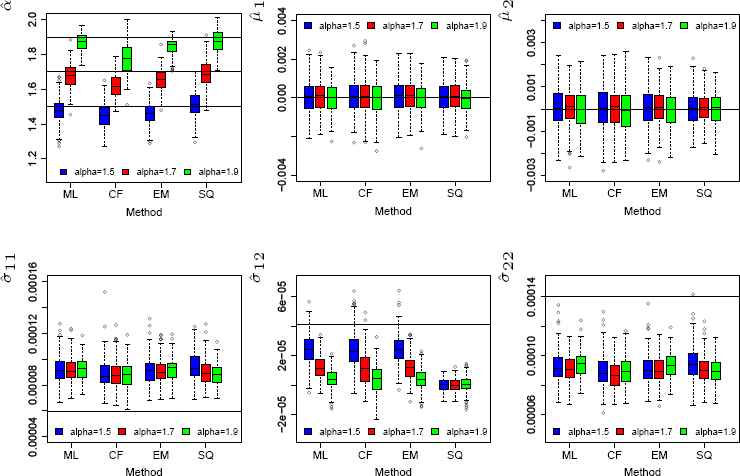
Boxplot of the ML, CF, EM, and SQ estimations for α, μ = (μ₁, μ₂)^T, and entries of Σ when n = 500 vectors generated from a bivariate sub-Gaussian SαS with α = 1.5, 1.7, 1.9, μ = (μ₁,μ₂)^T = (0,0)^T, σ₁₁ = 0.000059552, σ₁₂ = 0.000040783, and σ₂₂ = 0.000139861. In each sub-figure, horizontal line denotes the real value of parameter. Each boxplot is constructed based on N = 250 runs. The used color scheme under each method for boxplots is: blue, red, and green for α = 1.5, 1.7, and 1.9, respectively.

5.4. Real data analysis in bivariate case

Here, we apply ML, SQ, CF, and EM methods to S&P500 and IPC indices selected from WMI data set. The empirical distribution of both S&P500 and IPC indices show a symmetric pattern around the origin. The scatterplot shown in Figure 5 is roughly elliptical contoured. Furthermore, estimated tail parameters after fitting a stable distribution to S&P500 and IPC indices through the ML approach are 1.9003 and 1.9143, respectively, which are assumed to be equal. Thus, the assumption that X = (S&P500, IPC)^T follows a sub-Gaussian SαS distribution is acceptable, [23]. The results of estimating parameters through ML, CF, EM, and SQ methods are shown in Table 3. The log-likelihood values indicate that the EM algorithm gives better performance than the CF and SQ approaches.

5.5. Analysis in higher dimensions

In this subsection, firstly we perform a simulation to compare the performance of the ML, CF, EM, and SQ methods where a sample of size n = 1500 is generated from three-variate sub-Gaussian SαS distribution. For this purpose, the considered settings are: α = 1.86, μ = (μ₁, μ₂, μ₃)^T = (0, 0, 0)^T , and

which were used by [24]. Secondly, we fit a thirty-dimensional sub-Gaussian S S distribution to the 30 indices of Dow Jones data described in [24].

For three-variate case, results of the simulation are displayed in Figure 7 where each boxplot is based on 250 runs. If we define the length of each box as a performance criterion, it follows that the EM algorithm works better than the SQ method in all cases. The performance of the EM and CF approaches is almost the same except in the case of estimating α where the EM algorithm performs much better than the CF method. In the case of case of thirty-dimensional, implementing the EM algorithm takes 303 seconds when M = 200 and M₀ = 150. To avoid unnecessary details, we only focus on estimating the location parameter and diagonal entries of the dispersion matrix using the EM and ML methods. The result for estimating these parameters are given in Figures 8-9, respectively. As it is seen, the EM algorithm gives results close to the ML approach for estimating diagonal entries of the dispersion matrix. The results of simulation show that the computational cost increases as dimensions increase but differences are not significant. For example, the execution time for implementing the EM and ML methods are given in Table 4. For this, we generated n = 1000 random vectors of a sub-Gaussian SαS distribution.

Fig. 7.

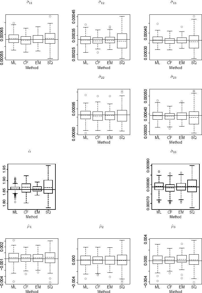
Boxplot of the ML, CF, EM, and SQ estimations for α, μ = (μ₁, μ₂, μ₃)^T, and entries of Σ when n = 1500 vectors generated from a three-variate sub-Gaussian SαS with α = 1.86, μ = (μ₁, μ₂, μ₃)^T = (0, 0, 0)^T, σ₁₁ = 0.0006293, σ₁₂ = 0.0003289, σ₁₃ = 0.0003643, σ₂₂ = 0.0009133, σ₂₃ = 0.0003921, and σ₃₃ = 0.0007871. In each sub-figure, horizontal line denotes the real value of parameter. Each boxplot is constructed based on N = 250 runs.

Fig. 8.

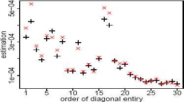
Estimated values for diagonal entries of dispersion matrix when the EM and ML methods are applied to 30 indices of Dow Jones data. The signs × and + correspond to the EM and ML methods.

Fig. 9.

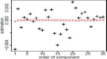
Estimated values for location parameter when the EM and ML methods are applied to 30 indices of Dow Jones data. The signs × and + correspond to the EM and ML methods.