
Parameter Estimation and Application of Generalized Inflated Geometric Distribution
- DOI
- 10.2991/jsta.2018.17.3.7How to use a DOI?
- Keywords
- Standardized bias; Standardized mean squared error; Akaike’s Information Criterion (AIC); Bayesian Information Criterion (BIC); Monte Carlo study
- Abstract
A count data that have excess number of zeros, ones, twos or threes are commonplace in experimental studies. But these inflated frequencies at particular counts may lead to overdispersion and thus may cause difficulty in data analysis. So to get appropriate results from them and to overcome the possible anomalies in parameter estimation, we may need to consider suitable inflated distribution. Generally, Inflated Poisson or Inflated Negative Binomial distribution are the most commonly used for modeling and analyzing such data. Geometric distribution is a special case of Negative Binomial distribution. This work deals with parameter estimation of a Geometric distribution inflated at certain counts, which we called Generalized Inflated Geometric (GIG) distribution. Parameter estimation is done using method of moments, empirical probability generating function based method and maximum likelihood estimation approach. The three types of estimators are then compared using simulation studies and finally a Swedish fertility dataset was modeled using a GIG distribution.
- Copyright
- © 2018, the Authors. Published by Atlantis Press.
- Open Access
- This is an open access article under the CC BY-NC license (http://creativecommons.org/licences/by-nc/4.0/).
1. Introduction
A random variable X that counts the number of trials to obtain the rth success in a series of independent and identical Bernoulli trials, is said to have a Negative Binomial distribution whose probability mass function (pmf) is given by
The above distribution is also the “Generalized Power Series distribution” as mentioned in Johnson et al. (2005) [9]. Some writers, for instance Patil et al. (1984) [12], called this the “Pólya-Eggenberger distribution”, as it arises as a limiting form of Eggenberger and Pólya’s (1923) [5] urn model distribution. A special case of Negative Binomial Distribution is the Geometric distribution which can be defined in two different ways
Firstly, the probability distribution for a Geometric random variable X (where X being the number of independent and identical trials to get the first success) is given by
However, instead of counting the number of trials, if the random variable X counts the number of failures before the first success, then it will result in the second type of Geometric distribution which again is a special case of Negative Binomial distribution when r = 1 (first success) and its pmf is given by
- •
The famous problem of Banach’s match boxes (Feller (1968) [6]);
- •
- •
A ticket control problem (Jagers (1973) [8]);
- •
A survillance system for congenital malformations (Chen (1978) [4]);
- •
The number of tosses of a fair coin before the first head (success) appears;
- •
The number of drills in an area before observing the first productive well by an oil prospector (Wackerly et al. (2008) [15]).
The Geometric model in (1.3) which is widely used for modeling count data may be inadequate for dealing with overdispersed count data. One such instance is the abundance of zero counts in the data, and (1.3) may be an inefficient model for such cases due to the presence of heterogeneity, which usually results in undesired over dispersion. Therefore, to overcome this situation, i.e., to explain or capture such heterogeneity, we consider a ‘two-mass distribution’ by giving mass π1 to 0 counts, and mass (1 − π1) to the other class which follows Geometric(p). The result of such a ‘mixture distribution’ is called the ‘Zero-Inflated Geometric’ (ZIG) distribution with the probability mass function
A further generalization of (1.4) can be obtained by inflating/deflating the Geometric distribution at several specific values. To be precise, if the discrete random variable X is thought to have inflated probabilities at the values k1, ...., km ∈ {0, 1, 2,.... }, then the following general probability mass function can be considered:
We will consider some special cases of the (GIG) distribution such as Zero-One-Inflated Geometric (ZOIG) distribution in the case k = 2 with k1 = 0 and k2 = 1 or Zero-One-Two Inflated Geometric (ZOTIG) models. Similar type of Generalized Inflated Poisson (GIP) models have been considered by Melkersson and Rooth (2000) [11] to study a women’s fertility data of 1170 Swedish women of the age group 46–76 years (Table 1). This data set consists of the number of child(ren) per woman, who have crossed the childbearing age in the year 1991. They justified the Zero-Two Inflated Poisson distribution was the best to model it. However recently, Begum et al. (2014) [2] studied the same data set and found that a Zero-Two-Three Inflated Poisson (ZTTIP) distribution was a better fit.
| Count | Frequency | Proportion |
|---|---|---|
| 0 | 114 | .097 |
| 1 | 205 | .175 |
| 2 | 466 | .398 |
| 3 | 242 | .207 |
| 4 | 85 | .073 |
| 5 | 35 | .030 |
| 6 | 16 | .014 |
| 7 | 4 | .003 |
| 8 | 1 | .001 |
| 10 | 1 | .001 |
| 12 | 1 | .001 |
|
|
||
| Total | 1,170 | 1.000 |
Observed number of children (= count) per woman.
Instead of using an Inflated Poisson model, we will consider fitting appropriate Inflated Geometric models to the data in Table 1. Now, which model is the best fit whether a GIG model with focus on counts (0, 1), i.e., ZOIG or a GIG model focusing on some other set {k1, k2,…, km} is appropriate for the above data will be eventually decided by different model selection criteria in section 5. The rest of the paper is organized as follows. In the next section, we provide some properties of the GIG distribution. In section 3, we discuss different techniques of parameter estimation namely, the method of moments (MME), empirical probability generating function (epgf) based methods (EPGE) suggested by Kemp and Kemp (1988) [10], and the maximum likelihood estimation (MLE). In section 4, we compare the performances of MMEs, EPGEs and MLEs for different GIG model parameters using simulation studies. Finally conclusion is given in section 6.
2. Some Properties
In this section, we present some properties of the GIG distribution and that of some special cases of this distribution.
Proposition 1.
The probability generating function (pgf) of a random variable X following a GIG in (1.5) with parameters π1,…, πm and p is given by
Proposition 2.
The rth raw moment of a random variable X following a GIG in (1.5) with parameters π1,…, πm and p is given by
Proof.
For the ZIG distribution, i.e., when m = 1 and k1 = 0, using (2.1) we get the pgf as
| π1 | p | ||||||||
|---|---|---|---|---|---|---|---|---|---|
|
|
|||||||||
| 0.1 | 0.2 | 0.3 | 0.4 | 0.5 | 0.6 | 0.7 | 0.8 | 0.9 | |
| 0.1 | 10.90 | 5.40 | 3.57 | 2.65 | 2.10 | 1.73 | 1.47 | 1.28 | 1.12 |
| 0.2 | 11.80 | 5.80 | 3.80 | 2.80 | 2.20 | 1.80 | 1.51 | 1.30 | 1.13 |
| 0.3 | 12.70 | 6.20 | 4.03 | 2.95 | 2.30 | 1.87 | 1.56 | 1.33 | 1.14 |
| 0.4 | 13.60 | 6.60 | 4.27 | 3.10 | 2.40 | 1.93 | 1.60 | 1.35 | 1.16 |
| 0.5 | 14.50 | 7.00 | 4.50 | 3.25 | 2.50 | 2.00 | 1.64 | 1.38 | 1.17 |
| 0.6 | 15.40 | 7.40 | 4.73 | 3.40 | 2.60 | 2.07 | 1.69 | 1.40 | 1.18 |
| 0.7 | 16.30 | 7.80 | 4.97 | 3.55 | 2.70 | 2.13 | 1.73 | 1.43 | 1.19 |
| 0.8 | 17.20 | 8.20 | 5.20 | 3.70 | 2.80 | 2.20 | 1.77 | 1.45 | 1.20 |
| 0.9 | 18.10 | 8.60 | 5.43 | 3.85 | 2.90 | 2.27 | 1.81 | 1.48 | 1.21 |
Var(X) / E(X) for ZIG distribution
The cumulative distribution function (cdf) of the ZIG distribution is given by
Using (1.5), the probability mass function of ’Zero-One-Inflated Geometric’ (ZOIG) distribution, i.e., when m = 2 and k1 = 0 and k2 = 1, can be obtained as
Also using (2.1), we obtain the pgf of ZOIG distribution as
3. Estimation of Model Parameters
In this section, we estimate the parameters by three well known methods of parameter estimation namely the method of moment estimations, methods based on empirical probability generating function and the method of maximum likelihood estimations.
3.1. Method of Moments Estimation (MME)
The easiest way to obtain estimators of the parameters is through the method of moments estimation (MME). Given a random sample X1,...., Xn, i.e. independent and identically distributed (iid) observations from the GIG distribution, we equate the sample moments with the corresponding population moments (2.2) to get a system of (m+1) equations involving the (m+1) model parameters p, π1,..., πm of the form
Consider the case of ZIG distribution when m = 1 i.e., k1 = 0, resulting into only two parameters to estimate, i.e. π1 and p. In order to obtain the method of moments estimators, we can equate the mean and variance given in (2.3) with sample mean (
Now let us consider another special case of GIG, the Zero-One Inflated Geometric (ZOIG) distribution, i.e., m = 2 and k1 = 0 and k2 = 1. It has three parameters π1, π2 and p and to estimate them we need to equate the first three raw sample moments with the corresponding population moments and we thus obtain the following system of equations:
Similarly, another special case of GIG is the Zero-One-Two Inflated Geometric (ZOTIG) distribution. Here we have four parameters π1, π2, π3 and p to estimate. This is done by solving the following system of four equations obtained by equating the first four raw sample moments with their corresponding population moments to have,
Algebraic solutions to these systems of equations in (3.4) and (3.5) are obtained by using Mathematica. We note that these solutions may not fall in the feasible regions of the parameter space, so we put appropriate restrictions to these solutions as discussed for the ZIG distribution to obtain the corrected MMEs.
3.2. Methods based on Probability Generating Function (EPGE)
Given a random sample X1, X2,…, Xn of size n from a distribution with pgf G(s), the empirical probability generating function (epgf) is defined as
3.3. Maximum Likelihood Estimation (MLE)
Now we discuss the approach of estimating our parameters by the method of Maximum Likelihood Estimation(MLE). Based on the random sample X = (X1, X2,..., Xn), we define the likelihood function L = L(p, πi, 1 ≤ i ≤ m | X) as follows. Let Yi = the number of observations at ki with inflated probability, i.e., if I is an indicator function, then
Usually, of the three methods discussed, MLE is known to work best but in absence of closed form expression we have to resort to numerical optimization techniques, which makes it the most difficult one to obtain. Using the other two methods (MME and EPGE), estimators are much easier to obtain and do not require extensive computation, but they may lie outside the feasibility region of the parameter space. So we need to appropriately correct them. Therefore, we conduct simulation studies in the next section which can provide some guidance about their performances.
4. Simulation Study
We have considered the following three cases for our simulation study:
- (i)
m = 1, k1 = 0 (Zero Inflated Geometric (ZIG) distribution)
- (ii)
m = 2, k1 = 0, k2 = 1 (Zero-One Inflated Geometric (ZOIG) distribution)
- (iii)
m = 3, k1 = 0, k2 = 1, k3 = 2 (Zero-One-Two Inflated Geometric (ZOTIG) distribution)
For each model mentioned above, we generate random data X1,..., Xn from the distribution (with given parameter values) N = 10,000 times. Let us denote a parameter (either πi or p) by the generic notation θ. The parameter θ is estimated by three possible estimators
Note that
4.1. The ZIG Distribution
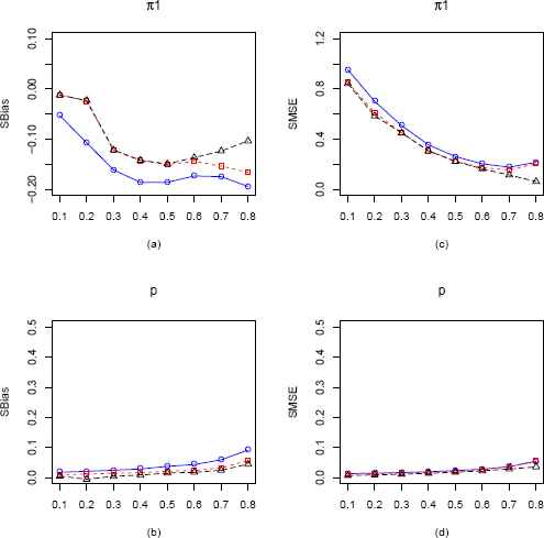
In our simulation study for the Zero Inflated Geometric (ZIG) distribution, we fix p = 0.2 and vary π1 from 0.1 to 0.8 with an increment of 0.1 for n = 25, 100. The constrained optimization algorithm “L-BFGS-B” (Byrd et al. (1995)) [3] is implemented in R programming language to obtain the maximum likelihood estimators (MLEs) of the parameters p and π1, and the corrected MMEs and EPGEs are obtained by solving a system of equations and imposing appropriate restrictions on the parameters. In order to compare the performances of the MLEs with that of the CMMEs and EPGEs, we plot the standardized biases (SBias) and standardized MSE (SMSE) of these estimators obtained over the allowable range of π1. The SBias and SMSE plots are presented in Figure 1 for sample size 25. Due to space constraint, the plot for sample size 100 is presented in Figure 8 in the Appendix. Also we have presented in the Appendix a plot when p = 0.7 and n = 100 (Figure 9).
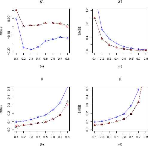
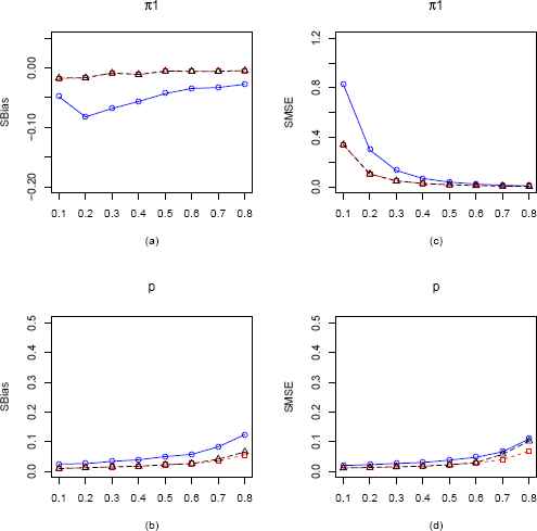
Plots of the SBias and SMSE of the CMMEs, EPGEs and MLEs of π1 and p (from ZIG distribution) plotted against π1 for p = 0.2 and n = 25. The solid blue line represents the SBias or SMSE of the CMME. The dashed red line represents the SBias or SMSE of the EPGE and the longdashed black line is for the MLE. (a) Comparison of SBias of π1 estimators. (b) Comparison of SBias of p estimators. (c) Comparison of SMSE of π1 estimators. (d) Comparison of SMSE of p estimators.
For the ZIG distribution with n = 25, from Figure 1(a) we see that MLE and EPGE outperforms CMME for all values of π1 with respect to SBias except at π1 = 0.1. All the estimators beyond 0.2 are negatively biased. In Figure 1(b), we again see that MLE and EPGE uniformly outperforms the CMME and are increasing with values of π1. In Figure 1(c), MLE and EPGE consistently outperforms CMME at all points w.r.t SMSE. For all the estimators, the SMSE starts off at their highest values and then decreases rapidly until it reaches nearly zero. The SMSE of MLE and EPGE consistently outperforms that of CMME in Figure 1(d). They both start off at their lowest values, and increase as values of π1 get higher. For n = 100, from Figure 8 we see a similar pattern. However, as expected the values of sBias and SMSE are considerably smaller for all estimators.
When p = 0.7, from Figure 9 we observe that MLE outperforms both CMME and EPGE. Again all estimators of π1 seems to be negatively biased and MLE and EPGE of p is almost unbiased up to π1 = 0.7. We also observe that SMSE of MLE for both the parameters π1 and p is smallest among the three estimators.
4.2. The ZOIG Distribution
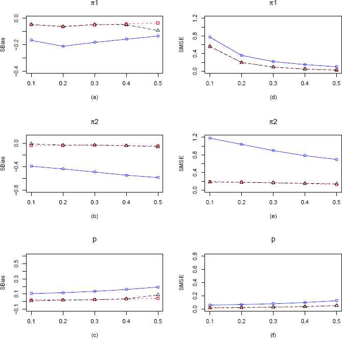
In the case of the Zero-One Inflated Geometric (ZOIG) distribution we have three parameters to consider, namely π1, π2 and p. For fixed p = 0.3 we vary π1 and π2 one at a time for sample sizes 25 and 100. Figure 2 presents the comparisons for the three different type of estimators for three parameters π1, π2 and p in terms of standardized bias and standardized MSE for n = 25, varying π1 from 0.1 to 0.5 and keeping π2 and p fixed at 0.15 and 0.3 respectively. Figure 10 in the Appendix presents the same for sample size 100. Also in the Appendix a plot when p is fixed at 0.7 and n = 100 is given in Figure 11. In Figure 2(a), both MLE and EPGE outperforms CMME at all points with respect to SBias. SBias of MLE and EPGE starts above zero and quickly becomes negative, whereas that of CMME is throughout negative. In Figure 2(b), we see that the MLE is almost unbiased for values of π1 up to 0.4, and SBias of both CMME and EPGE are always negative. Again in Figure 2(c), we see that MLE outperforms both CMME and EPGE. In Figure 2(d), SMSE of all the estimators are decreasing, but SMSE of MLE stays below that of other two estimators. In Figure 2(e), SMSE of MLE stays constant at 0.55 and in 2(f), SMSE of MLE stays below that of the other estimators.
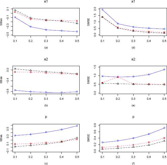
Plots of the SBias and SMSE of the CMMEs, EPGEs and MLEs of π1, π2 and p (from ZOIG distribution) by varying π1 for fixed π2 = 0.15, p = 0.3 and n = 25. The solid blue line represents the SBias or SMSE of the corrected MME. The dashed red line and longdashed black line represents the SBias or SMSE of the EPGE and MLE respectively. (a)–(c) Comparisons of SBiases of π1, π2 and p estimators respectively. (d)–(f) Comparisons of SMSEs of π1, π2 and p estimators respectively.
For sample size n = 100 from Figure 10, we observe that both MLE and EPGE for all the parameters are almost unbiased and performs better than CMME. However, SMSE wise MLE is marginally better. We also observe that with the increase in sample size the SBias and SMSE of all the estimators have gone down.
When p = 0.7 and n = 100, from Figure 11 we observe that SBias of π1 is decreasing for all the estimators. However for π2, SBias of MLE starts of with very small positive value and then becomes negative, whereas both EPGE and CMME are negatively biased and MLE is almost unbiased for parameter p. Also SMSE wise, MLE seems to be the best estimator.
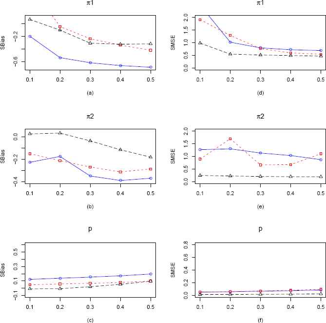
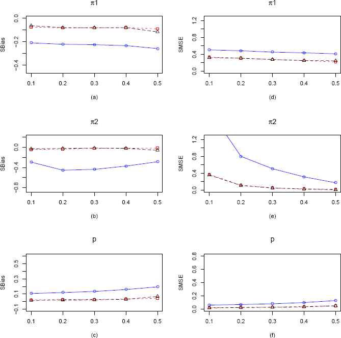
In our second scenario which is presented in Figure 3 for sample size 25, we vary π2 keeping π1 and p fixed at 0.15 and 0.3 respectively. Figure 12 in the Appendix contains the same plots for sample size 100. Also in the Appendix we present comparison plots of SBias and SMSE in Figure 13 for sample size 100, varying π2 keeping π1 and p fixed at 0.15 and 0.7 respectively. In Figure 3(a), we see that all three estimators are negatively biased, but MLE is always performing better. However in Figure 3(b), MLE starts of with a positive bias and then becomes almost unbiased for π2. SBias of EPGE is negative throughout but stays very close 0. SBias of CMME stays throughout between −0.6 and −0.8. In Figure 3(c), we see that MLE outperforms both CMME and EPGE throughout with respect to SBias. From Figures 3(d), 3(e) and 3(f), it is clear that MLE outperforms both CMME and EPGE with respect to SMSE for all permissible values of π2. Thus we observe that the MLEs of the all three parameters perform better in terms of the both SBias and SMSE.
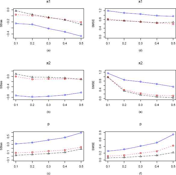
Plots of the SBias and SMSE of the CMMEs, EPGEs and MLEs of π1, π2 and p (from ZOIG distribution) by varying π2 for fixed π1 = 0.15, p = 0.3 and n = 25. The solid blue line represents the SBias or SMSE of the corrected MME. The dashed red line and longdashed black line represents the SBias or SMSE of the EPGE and MLE respectively. (a)–(c) Comparisons of SBiases of π1, π2 and p estimators respectively. (d)–(f) Comparisons of SMSEs of π1, π2 and p estimators respectively.
We observe very similar behavior from the plots for n = 100, presented in Figure 12. MLE seems to be performing best and SBias and SMSEs are going down as expected with an increase in sample size except for SMSE of π2 (Figure 12(e)).
Again from Figure 13, when p = 0.7 and n = 100, we observe that MLE is performing better than EPGE and CMME w.r.t both SBias and SMSE.
4.3. The ZOTIG Distribution
For the Zero-One-Two Inflated Geometric (ZOTIG) distribution we have four parameters to consider, namely π1, π2, π3 and p. For fixed p = 0.3 we vary π1, π2, and π3 one at a time from 0.1 to 0.5 for sample size n = 25. Thus we have 12 estimators
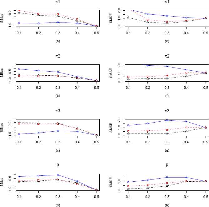
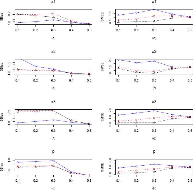
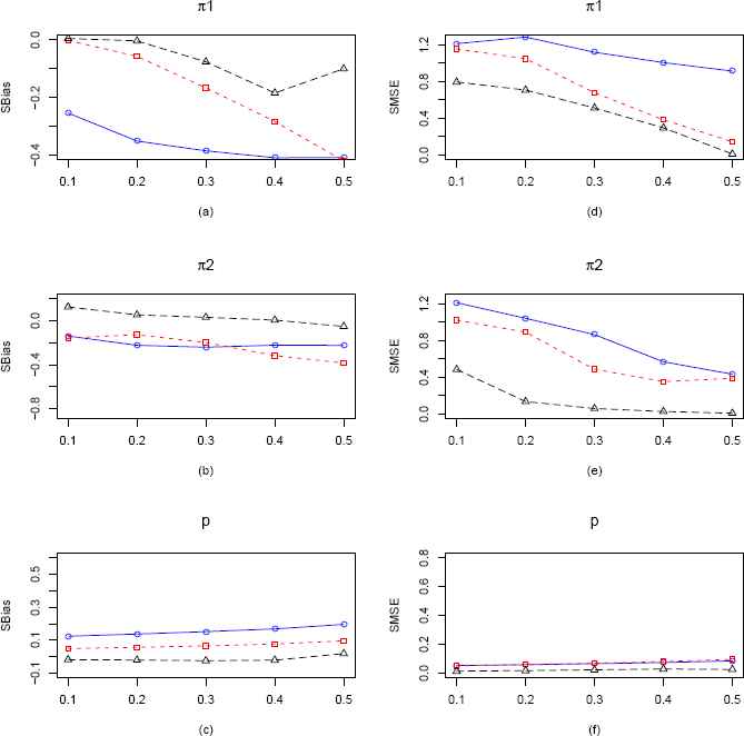
Plots of the SBias and SMSE of the CMMEs, EPGEs and MLEs of π1, π2, π3 and p (from ZOTIG distribution) by varying π1 for fixed π2 = π3 = 0.2 and p = 0.3 and n = 25. The solid blue line represents the SBias or SMSE of the corrected MME. The dashed red line and longdashed black line represents the SBias or SMSE of the EPGE and MLE respectively. (a)–(d) Comparisons of SBiases of π1, π2, π3 and p estimators respectively. (e)–(h) Comparisons of SMSEs of π1, π2, π3 and p estimators respectively.
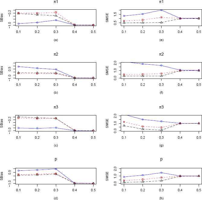
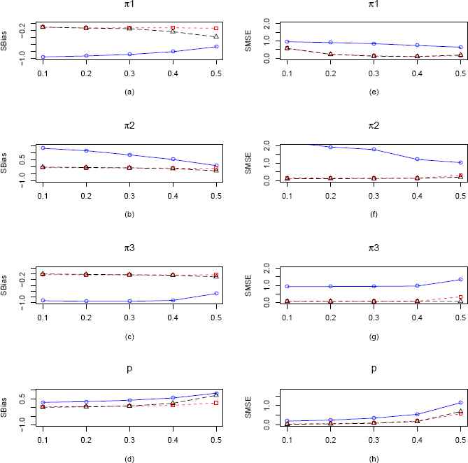
Plots of the SBias and SMSE of the CMMEs and MLEs of π1, π2, π3 and p (from ZOTIG distribution) by varying π2 for fixed π1 = π3 = 0.2 and p = 0.3 and n = 25. The solid blue line represents the SBias or SMSE of the corrected MME. The dashed red line and longdashed black line represents the SBias or SMSE of the EPGE and MLE respectively. (a)–(d) Comparisons of SBiases of π1, π2, π3 and p estimators respectively. (e)–(h) Comparisons of SMSEs of π1, π2, π3 and p estimators respectively.
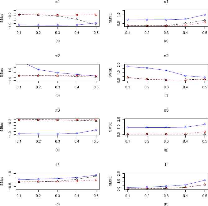
Plots of the SBias and SMSE of the CMMEs and MLEs of π1, π2, π3 and p (from ZOTIG distribution) by varying π3 for fixed π1 = π2 = 0.2 and p = 0.3 and n = 25. The solid blue line represents the SBias or SMSE of the corrected MME. The dashed red line and longdashed black line represents the SBias or SMSE of the EPGE and MLE respectively. (a)–(d) Comparisons of absolute SBiases of π1, π2, π3 and p estimators respectively. (e)–(h) Comparisons of SMSEs of π1, π2, π3 and p estimators respectively.
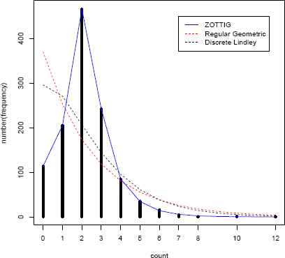
Plot of the observed frequencies compared to the estimated frequencies from the regular Geometric, discrete Lindley and the Zero-One-Two-Three Inflated Geometric model.
Plots of the SBias and SMSE of the CMMEs, EPGEs and MLEs of π1 and p (from ZIG distribution) plotted against π1 for p = 0.2 and n = 100. The solid blue line represents the SBias or SMSE of the CMME. The dashed red line represents the SBias or SMSE of the EPGE and the longdashed black line is for the MLE. (a) Comparison of SBias of π1 estimators. (b) Comparison of SBias of p estimators. (c) Comparison of SMSE of π1 estimators. (d) Comparison of SMSE of p estimators.
Plots of the SBias and SMSE of the CMMEs, EPGEs and MLEs of π1 and p (from ZIG distribution) plotted against π1 for p = 0.7 and n = 100. The solid blue line represents the SBias or SMSE of the CMME. The dashed red line represents the SBias or SMSE of the EPGE and the longdashed black line is for the MLE. (a) Comparison of SBias of π1 estimators. (b) Comparison of SBias of p estimators. (c) Comparison of SMSE of π1 estimators. (d) Comparison of SMSE of p estimators.
Plots of the SBias and SMSE of the CMMEs, EPGEs and MLEs of π1, π2 and p (from ZOIG distribution) by varying π1 for fixed π2 = 0.15, p = 0.3 and n = 100. The solid blue line represents the SBias or SMSE of the corrected MME. The dashed red line and longdashed black line represents the SBias or SMSE of the EPGE and MLE respectively. (a)–(c) Comparisons of SBiases of π1, π2 and p estimators respectively. (d)–(f) Comparisons of SMSEs of π1, π2 and p estimators respectively.
Plots of the SBias and SMSE of the CMMEs, EPGEs and MLEs of π1, π2 and p (from ZOIG distribution) by varying π1 for fixed π2 = 0.15, p = 0.7 and n = 100. The solid blue line represents the SBias or SMSE of the corrected MME. The dashed red line and longdashed black line represents the SBias or SMSE of the EPGE and MLE respectively. (a)–(c) Comparisons of SBiases of π1, π2 and p estimators respectively. (d)–(f) Comparisons of SMSEs of π1, π2 and p estimators respectively.
Plots of the SBias and SMSE of the CMMEs, EPGEs and MLEs of π1, π2 and p (from ZOIG distribution) by varying π2 for fixed π1 = 0.15, p = 0.3 and n = 100. The solid blue line represents the SBias or SMSE of the corrected MME. The dashed red line and longdashed black line represents the SBias or SMSE of the EPGE and MLE respectively. (a)–(c) Comparisons of SBiases of π1, π2 and p estimators respectively. (d)–(f) Comparisons of SMSEs of π1, π2 and p estimators respectively.
Plots of the SBias and SMSE of the CMMEs, EPGEs and MLEs of π1, π2 and p (from ZOIG distribution) by varying π2 for fixed π1 = 0.15, p = 0.7 and n = 100. The solid blue line represents the SBias or SMSE of the corrected MME. The dashed red line and longdashed black line represents the SBias or SMSE of the EPGE and MLE respectively. (a)–(c) Comparisons of SBiases of π1, π2 and p estimators respectively. (d)–(f) Comparisons of SMSEs of π1, π2 and p estimators respectively.
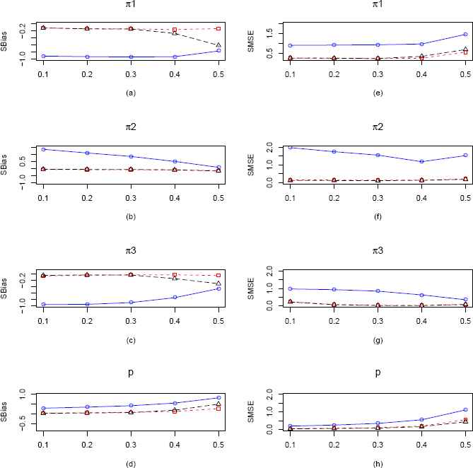
Plots of the SBias and SMSE of the CMMEs, EPGEs and MLEs of π1, π2, π3 and p (from ZOTIG distribution) by varying π1 for fixed π2 = π3 = 0.2 and p = 0.3 and n = 100. The solid blue line represents the SBias or SMSE of the corrected MME. The dashed red line and longdashed black line represents the SBias or SMSE of the EPGE and MLE respectively. (a)–(d) Comparisons of SBiases of π1, π2, π3 and p estimators respectively. (e)–(h) Comparisons of SMSEs of π1, π2, π3 and p estimators respectively.
Plots of the SBias and SMSE of the CMMEs, EPGEs and MLEs of π1, π2, π3 and p (from ZOTIG distribution) by varying π2 for fixed π1 = π3 = 0.2 and p = 0.3 and n = 100. The solid blue line represents the SBias or SMSE of the corrected MME. The dashed red line and longdashed black line represents the SBias or SMSE of the EPGE and MLE respectively. (a)–(d) Comparisons of SBiases of π1, π2, π3 and p estimators respectively. (e)–(h) Comparisons of SMSEs of π1, π2, π3 and p estimators respectively.
Plots of the SBias and SMSE of the CMMEs, EPGEs and MLEs of π1, π2, π3 and p (from ZOTIG distribution) by varying π3 for fixed π1 = π2 = 0.2 and p = 0.3 and n = 100. The solid blue line represents the SBias or SMSE of the corrected MME. The dashed red line and longdashed black line represents the SBias or SMSE of the EPGE and MLE respectively. (a)–(d) Comparisons of SBiases of π1, π2, π3 and p estimators respectively. (e)–(h) Comparisons of SMSEs of π1, π2, π3 and p estimators respectively.
In the first scenario of ZOTIG distribution, which is presented in Figure 4, we vary π1 keeping π2, π3 and p fixed at 0.2, 0.2 and 0.3 respectively. From Figure 4(a, b, c, d), we see that the CMMEs of all the four parameters perform consistently worse than the MLEs and EPGEs with respect to SBias. Both MLEs and EPGEs seems to have very similar performance. Also from parts (e, f, g, h) in Figure 4 concerning the SMSE, we notice that the MLEs of all the parameters perform consistently better than the other two type of estimators. We observe similar performance of the three types of estimators, when sample size is increased to 100 (Figure 14).
In our second scenario which is presented in Figure 5, we vary π2 keeping π1, π3 and p fixed at 0.2, 0.2 and 0.3 respectively. We observe some interesting things in these plots. From Figure 5 we see that MLE and EPGE of π1, π2, π3 and p are performing better upto π2 = 0.4 with respect to SBias but after that performance of all the estimators are same. However we see that the MLEs of all four parameters perform better than their CMME and EPGE counterparts with respect to SMSE. In Figure 15, when sample size is 100, we observe that CMMEs are consistently worse w.r.t both SBias and SMSE and EPGEs are performing marginally better than MLEs.
In the third scenario which is presented in Figure 6, we vary π3 keeping π1, π2 and p fixed at 0.2, 0.2 and 0.3 respectively. Here also we observe similar results as the second case of ZOTIG distribution, MLEs and EPGEs for all the four parameters are uniformly outperforming CMMEs with respect to SBias up to π3 = 0.4. Also as before MLEs uniformly outperform CMMEs and EPGEs of all the four parameters with respect to SMSE. But as sample size increases to 100, we observe that EPGEs are performing marginally better than MLEs (Figure 16).
Thus from our simulation study it is evident that MLE has an overall better performance than CMME and EPGE for all the Generalized Inflated Geometric models that we have considered. So in the next chapter, we consider an example where we fit an appropriate GIG model to the Swedish fertility data set.
5. Application of GIG Distribution
In this section, we consider the Swedish fertility data presented in Table 1 and try to fit a suitable GIG model. Since our simulation study in the previous section suggests that the MLE has an overall better performance, all of our estimations of model parameters are carried out using the maximum likelihood estimation approach. While fitting the Inflated Geometric models, parameter estimates of some mixing proportions (πi) came out negative. So we need to make sure that all the estimated probabilities according to the fitted models are non-negative. We tried all possible combinations of GIG models and then compared each of these Inflated Geometric models using the Chi-square goodness of fit test, the Akaike’s Information Criterion (AIC) and the Bayesian Information Criterion (BIC). While performing the Chi-square goodness of fit test, the last three categories of Table 1 are collapsed into one group due to small frequencies. More details of our model fitting is presented below.
First, we try with single-point inflation at each of the four values (0, 1, 2 and 3). In this first phase, an inflation at 2 seems most plausible as it gives the smallest AIC and BIC values 4188.794 and 4198.924 respectively. However the p-value of the Chi-square test is very close to 0, suggesting that this is not a good model. Next, we try two-point inflations at {0, 1}, {0, 2}, {0, 3}, {1, 2}, etc. At this stage, {2, 3} inflation seems most appropriate going by the values of AIC (3947.064) and BIC ( 3962.258). But p-value of the Chi-square test close to 0 again makes it an inefficient model.
In the next stage, we try three-point inflation models, and here we note that a GIG with inflation set {0, 2, 3} significantly improves over the earlier {2, 3} inflation model (i.e., TTIG). This ZTTIG model significantly improves the p-value (but still close to 0) while maintaining a low AIC and BIC of 3841.169 and 3861.428 respectively. The main reason for low p-value is that this model is unable to capture the tail behavior. The estimated value of the parameters are (with k1 = 0,k2 = 2,k3 = 3):
Finally, we fitted the full {0, 1, 2, 3} inflated model. We obtained the maximum likelihood estimates of the model parameters as
6. Conclusion
This work deals with a general inflated geometric distribution (GIG) which can be thought of as a generalization of the regular Geometric distribution. This type of distribution can effectively model datasets with elevated counts. We have discussed some properties of this distribution and also outlined the parameter estimation procedure for this distribution using the method of moments estimation, empirical probability generating function bases methods and the maximum likelihood estimation techniques. Simulation studies were also performed and we found that MLEs performed better than the corrected MMEs and EPGEs in estimating the model parameters with respect to the standardized bias (SBias) and standardized mean squared errors (SMSE). While performing the simulation, we observed that for certain ranges of the inflated proportions in the GIG models, the MMEs and EPGEs lie outside the parameter space. Nonetheless, we selected all permissible values and compared the overall performance of the CMMEs, EPGEs and MLEs for three special cases of GIG. Different GIG models were used for analyzing the fertility data of Swedish women and was compared with a discrete Lindley model. It was found that the Zero-One-Two-Three inflated Geometric (ZOTTIG) model is a good fit. Because of the extra parameter(s), the GIG distribution seems to be much more flexible in model fitting than the regular geometric distribution.
Acknowledgment
The authors are grateful to the editor and two referees for providing valuable comments and suggestions, which enhanced this work substantially.
Appendix A.
The probability mass function of the discrete Lindley distribution is given by
References
Cite this article
TY  - JOUR
AU  - Avishek Mallick
AU  - Ram Joshi
PY  - 2018
DA  - 2018/09/30
TI  - Parameter Estimation and Application of Generalized Inflated Geometric Distribution
JO  - Journal of Statistical Theory and Applications
SP  - 491
EP  - 519
VL  - 17
IS  - 3
SN  - 2214-1766
UR  - https://doi.org/10.2991/jsta.2018.17.3.7
DO  - 10.2991/jsta.2018.17.3.7
ID  - Mallick2018
ER  -