
f-Majorization with Applications to Stochastic Comparison of Extreme Order Statistics
- DOI
- 10.2991/jsta.2018.17.3.8How to use a DOI?
- Keywords
- Stochastic order; Exponentiated scale model; Frèchet distribution; Majorization; f-majorization order; Archimedean copula
- Abstract
In this paper, we use a new partial order, called f-majorization order. The new order includes as special cases the majorization, the reciprocal majorization and the p-larger orders. We provide a comprehensive account of the mathematical properties of the f-majorization order and give applications of this order in the context of stochastic comparison for extreme order statistics of independent samples following the Frèchet distribution and scale model. We discuss stochastic comparisons of series systems with independent heterogeneous exponentiated scale components in terms of the usual stochastic order and the hazard rate order. We also derive new result on the usual stochastic order for the largest order statistics of samples having exponentiated scale marginals and Archimedean copula structure.
- Copyright
- © 2018, the Authors. Published by Atlantis Press.
- Open Access
- This is an open access article under the CC BY-NC license (http://creativecommons.org/licences/by-nc/4.0/).
1. Introduction
In the modern life, applications of order statistics can be found in numerous fields, for example in statistical inference, life testing and reliability theory. The first important work devoted to the stochastic comparisons of order statistics arising from heterogeneous exponential random variables is the one by Pledger and Proschan [33]. Some other papers in this direction, and in particular devoted to the comparison of extreme order statistics from heterogeneous exponential distributions are [12], [34], [19]. There are many other papers on the comparison of extreme order statistics for some other models of parametric distributions. For example [21], [36], [25] and [38] deal with the case of heterogeneous Weibull distributions, [16] and [23] deal with with the case of heterogeneous exponentiated Weibull distributions, [3] deals with the case of heterogeneous generalized exponential distributions and [17] deals with the case of heterogeneous Frèchet distributions. A recent review on the topic can be also found in [4].
In these applications, various notions of majorization are used very often. The majorization orders which are used for finding some nice and applicable inequalities is also useful in understanding the insight of the theory. This concept deals with the diversity of the components of a vector in ℝn. Another interesting weaker order related to the majorization orders introduced in [9] is the p-larger order. In [40] the reciprocal majorization is introduced. Note that, for basic notation and terminologies on majorization where we use in this paper, we shall follow [28]. Fang and Zhang [15] and Fang [13] used a notion of majorization to prove Slepian’s inequality. In this paper, we use this notion, (called f-majorization order) and give applications of this order in the context of stochastic comparison of parallel/series systems with independent and dependent components. This notion includes as particular cases some of the previous ones.
The paper is organized as follows. In Section 2 we provide several notions of stochastic orders and majorization orders, and some known results. We also review notion of f -majorization, and then we present the the relationships with the previous notions and some new lemmas that will be used later. In Section 3 we provide new results for the comparison of extreme order statistics from heterogeneous Frèchet, scale and the exponentiated scale populations. We also derive new result on the usual stochastic order for the largest order statistics of the random samples having exponentiated scale marginals and Archimedean copula structure. To finish some conclusions are provided in Section 4.
Throughout this paper, we use the notations ℝ = (−∞, +∞), ℝ+ = [0, +∞) and ℝ++ = (0, +∞) and the term increasing means nondecreasing and decreasing means nonincreasing. Also the notation X1:n (Xn:n) is used to denote the smallest (largest) order statistic of n random variables X1,...,Xn. For any differentiable function f(·), we write f′(·) to denote the first derivative. The random variables considered in this paper are all nonnegative.
2. Preliminaries on majorization and new definitions
In this section, we recall some notions of stochastic orders, majorization and related orders and some useful lemmas, which are helpful for proving our main results.
Let X and Y be univariate random variables with distribution functions F and G, density functions f and g, survival functions
Definition 2.1.
Let X and Y be two random variables with common support ℝ++. The random variable X is said to be smaller than Y in the
- (i)
dispersive order, denoted by X ≤disp Y, if F−1(β) −F−1(α) ≤ G−1(β) −G−1(α) for all 0 < α ≤ β < 1,
- (ii)
hazard rate order, denoted by X ≤hr Y, if rF(x) ≥ rG(x) for all x,
- (iii)
reverse hazard rate order, denoted by X ≤rh Y, if
- (iv)
usual stochastic order, denoted by X ≤st Y, if
A real function ϕ is n-monotone on (a, b) ⊆ ℝ if (−1)n−2 ϕ(n−2) is decreasing and convex in (a, b) and (−1)k ϕ(k)(x) ≥ 0 for all x ∈ (a, b), k = 0, 1,...,n − 2, in which ϕ(i)(.) is the ith derivative of ϕ(.). For a n-monotone (n ≥ 2) function ϕ : ℝ+ → [0, 1] with ϕ(0) = 1 and limx→+∞ ϕ(x) = 0, let ψ = ϕ, −1 be the pseudo-inverse, then
Next we provide formal definitions of the different majorization notions that can be found in the literature. Note that, for basic notation and terminologies on majorization used in this paper, we shall follow [28]. To provide these notions, let us recall that the notation x(1) ≤ x(2) ≤ ... ≤ x(n) (x[1] ≥ x[2] ≥ ... ≥ x[n]) is used to denote the increasing (decreasing) arrangement of the components of the vector x = (x1,...,xn).
Definition 2.2.
The vector x is said to be
- (i)
weakly submajorized by the vector y (denoted by x ≼w y) if
- (ii)
weakly supermajorized by the vector y (denoted by
- (iii)
majorized by the vector y (denoted by
- (iv)
A vector x in
x is said to be log-majorized by y (denoted by
- (v)
A vector x in
- (vi)
A vector x in
The ordering introduced in definition 2.2 (iv), called log-majorization, was defined by Weyl [39] and studied by Ando and Hiai [1], who delved deeply into applications in matrix theory. Note that weak log-majorization implies weak submajorization. See 5.A.2.b. of [28]. Bon and Păltănea [9] and Zhao and Balakrishnan [40] introduced the order of p-larger and reciprocal majorization, Respectively. Here it should be noted that, for two vectors x and y, we have
It is well-known that (cf. [20] and [22])
The following lemma is needed for proving the main result.
Lemma 2.1.
(Balakrishnan et al. [3]). Let the function h : (0, ∞) × (0, 1) → (0, ∞) be defined as
Then,
- (i)
for each 0 < α ≤ 1, h(α, t) is decreasing with respect to t;
- (ii)
for each α ≥ 1, h(α, t) is increasing with respect to t.
We now introduce the main tool for this work. The idea is to use the new majorization notion, used by Fang and Zhang [15] and Fang [13], that includes as particular cases some of the previous ones. Also it will be used to provide some new results for the comparison of extreme values for the Frèchet distribution, scale, and the exponentiated scale model.
Definition 2.3.
Let f : 𝔸 → ℝ be a real valued function. The vector x is said to be
- (i)
weakly f-submajorized by the vector y, denoted by x ≼wf y, if f(x) ≼w f(y)
- (ii)
weakly f-supermajorized by the vector y, denoted by
- (iii)
f-majorized by the vector y, denoted by
It is easy to see that most of the previous majorization notions are examples of the previous notion for some particular choices of the function f . In particular we have:
The following lemma show the relation between f-majorization notion and usual majorization for various functions.
Lemma 2.2.
- (i)
If an increasing function f is convex, then
- (ii)
If an increasing function f concave, then x ≼wf y implies x ≼w y.
Proof.
The proof of this lemma follows easily from Theorem 5.A.2 of [28].
According to Lemma 2.2, all of the results which obtain for weak majorization are also true for f-majorization.
An interesting special case of Definition 2.3 by taking the exponential function can be achieved. More precisely, we have the following definition.
Definition 2.4.
A vector x in
Note that weak sub-majorization implies weak exp-majorization. See 5.A.2.g. of [28]. In the following example we see that weak exp-majorization does not imply weak sub-majorization.
Example 2.1.
Let (x1, x2) = (0.5, 0.9) and (y1, y2) = (1.08, 0.3). Obviously (x1, x2) ⋡w (y1, y2) and (y1, y2) ⋡w (x1, x2), even though we have
Next we provide an example, which shows that
Example 2.2.
Let
The following example shows that
Example 2.3.
Let x = (2, 3) and y = (1, 5), and f be any increasing function that assigns −5, 1.5, −4,1 to 1, 5, 2, 3, respectively. We observe that
Next we provide a set of technical results that will be used along the paper. First we introduce a lemma, which will be needed to prove our main results and is of interest in its own right.
Lemma 2.3.
The function
- (i)
if and only if, φ(f−1(a1),..., f−1(an)) is Schur-convex in (a1,...,an) and increasing (decreasing) in ai, for i = 1,...,n,
- (ii)
if and only if, φ(f−1(a1),..., f−1(an)) is Schur-convex (Schur-concave) in (a1,...,an), where ai = f (xi), for i = 1,...,n and f−1(y) = inf{x | f(x) ≥ y}.
Proof.
- (i)
Using definition 2.3, we see that (2.3) is equivalent to
where ai = f(xi) and bi = f(yi), for i = 1,...,n. Takingin Theorem 3.A.8 of [28], we get the required result. - (ii)
This case can be proved in a very similar manner.
It is noteworthy that Lemma 2.1 provided by Khaledi and Kochar [20] is a special case of Lemma 2.3 (i) when f(x) = log(x) and is useful for proving stochastic orders, see [18] and [3]. Recall that a real valued function φ defined on a set 𝒜 ∈ ℝn is said to be Schur-convex (Schur-concave) on 𝒜 if
3. Applications to the comparison of extreme order statistics
In this section we provide new results for the comparison of extreme values from independent Frèchet distribution, scale and exponentiated scale model. We also derive new result on the usual stochastic order for largest order statistics of samples having exponentiated scale marginals and Archimedean copula structure. As we will see the main tools are the new f-majorization notions introduced in the previous section.
3.1. Comparison of extreme order statistics for the Frèchet distribution
A random variable X is said to be distributed according to the Frèchet distribution, and will be denoted by X ~ Frè(µ, λ, α), if the distribution function is given by
In this section, we discuss stochastic comparisons of series and parallel systems with Frèchet distributed components in terms of the hazard rate order and the reverse hazard rate order. The result established here strengthens and generalizes some of the results of [17]. To begin with we present a generalization of Theorem 2 of [17] where sufficient condition is based on the weak f-majorization. This theorem provides the stochastic comparison result for the lifetime of the parallel systems having independently distributed Frèchet components with varying scale parameters, but fixed location and shape parameters.
Theorem 3.1.
Let X1,...,Xn (
- (i)
If (f−1(·))′( f−1(·))α−1 is increasing (decreasing) and
- (ii)
If (f−1(·))′( f−1(·))α−1 is decreasing (increasing) and (
Proof.
- (i)
Let us consider a fixed x > 0, and a strictly monotone function f, then the reversed hazard rate of Xn:n is given by
From Lemma 2.3, the proof follows if we prove that, for each x > 0,
Let h(ai) = α(x − µ)−α−1(f−1(ai))α. By the assumption, f is a strictly decreasing (increasing) function, therefore we have
Hence the reverse hazard rate function of Xn:n is decreasing (increasing) in each ai.
Now, from Proposition 3.C.1 of [28], the Schur-convexity (Schur-concavity) of
This completes the proof of the required result.
- (ii)
The proof is similar to the proof of part (i) and hence is omitted.
Let us describe some particular cases of previous theorem.
In Theorem 3.1. if we let
Corollary 3.1.
Let X1,...,Xn (
In Theorem 3.1. if we let f(x) = xr, r > 0, we can easily get the following result.
Corollary 3.2.
Let X1,...,Xn (
- (i)
If α ≥ r, and
- (ii)
If 0 < α ≤ r and
In the next corollary, which is an immediate consequence of Corollary 3.2, we discuss the stochastic comparison of two maximum order statistics, one from a heterogeneous population and the other one from a homogeneous population. Heterogeneity (or homogeneity) of a population is considered with respect to the scale parameters.
Corollary 3.3.
Let X1,...,Xn (
- (i)
If α ≥ r, and
- (ii)
If 0 < α ≤ r and
The first (second) part of the above Corollary gives a lower (upper) bound on the reversed hazard rate function of a parallel system with non-identical components in terms of the one with i.i.d. components when the common scale parameter is
The following theorem present a generalization of Theorem 1 of [17] where sufficient condition is based on the weak submajorization and by Lemma 2.2 (ii) is true under weak f submajorization for any increasing concave function f of the location parameters.
Theorem 3.2.
Let X1,...,Xn (
Proof.
It can be seen that the reversed hazard rate of Xn:n is given by
From Theorem 3.A.8 of [28], the proof follows if we prove that
Let
Therefore the reverse hazard rate function of Xn:n is increasing in each µi.
Now, from Proposition 3.C.1 of [28], we only need to prove the convexity of h to get the Schur-convexity of
In this case, we have that
Therefore we have that h is a convex function. This completes the proof.
Note that
3.2. Comparison of extreme values for scale model
Independent random variables X1,...,Xn are said to belong to the scale family of distributions if Xi ~ G(λix) where λi > 0, i = 1,...,n and G is called the baseline distribution and is an absolutely continuous distribution function with density function g. In the Theorem 3.3 we extend result of Theorem 2.1 of [18] to the case when the two sets of scale parameters weakly majorize each other instead of usual majorization which by Lemma 2.2 is true under weak f majorization of the scale parameters.
Theorem 3.3.
Suppose Xi and
- (i)
- (ii)
if r(x) is decreasing then
Proof.
- (i)
Fix x > 0. Then the hazard rate of X1:n is
where φ(u) = ur(u), u ≥ 0. From Theorem 3.A.8 of [28], it suffices to show that, for each x > 0, rX1:n(x, λ) is Schur-concave (Schur-convex) and increasing in λi’s. By the assumptions, φ(u) is increasing in u, then the hazard rate function of X1:n is increasing in each λi.Now, from Proposition 3.C.1 of [28], the concavity (convexity) of φ(λix) is needed to prove Schur-concavity (Schur-convexity) of rX1:n(x, λ). Note that the assumption that u2r′(u) is decreasing (increasing) in u is equivalent to r(u) + ur′(u) is decreasing (increasing) in u since
and r(u)+ur′(u) is decreasing (increasing) in u is equivalent to ur(u) is concave (convex) in u sinceHence, φ(u) is concave (convex). This completes the proof of part (i). - (ii)
Note that the conditions of Theorem 3.3 are satisfied by the generalized gamma distribution as [18] proved that for X ~ GG(p, q), xr(x) is an increasing function of x and x2r′(x) is an increasing function of x when p, q > 1 and is a decreasing function of x when p, q < 1. Recall that a random variable X has a generalized gamma distribution, denoted by X ~ GG(p, q), when its density function has the following form
Lastly, we get some new results on the lifetimes of parallel systems in terms of the usual stochastic order. It is noteworthy that [18] in Theorem 2.1 proved Theorem 3.4 when f (x) = log(x) and [19] in Theorem 2.2 proved Theorem 3.4 when the baseline distribution in the scale model is exponential and f (x) = log(x).
Theorem 3.4.
Let X1,...,Xn be a set of independent nonnegative random variables with Xi ~ G(λix), i = 1,...,n. Let
Proof.
The survival function of Xn:n can be written as
The assumption
3.3. Comparison of extreme values for exponentiated scale model
Recall that random variable X belongs to the exponentiated scale family of distributions if X ~ H(x) = [G(λx)]α, where α, λ > 0 and G is called the baseline distribution and is an absolutely continuous distribution function. We denote this family by ES(α, λ). Bashkar et al. [6] discussed stochastic comparisons of extreme order statistics from independent heterogeneous exponentiated scale samples. In this section, we provide new results for the comparison of smallest order statistics from samples following exponentiated scale model. In the following theorem, we compare series systems with independent heterogeneous ES components when one of the parameters is fixed, and the results are then developed with respect to the other parameter. Again by Lemma 2.2, this result is true under weak f-supermajorization where f is a non-negative strictly increasing convex function.
Theorem 3.5.
Let X1,...,Xn (
Proof.
Fix x > 0. Then the hazard rate of X1:n is
Recall that, a random variable X is said to be distributed according the generalized exponential distribution, and will be denoted by X ~ GE(α, λ), if the distribution function is given by
Corollary 3.4.
For i = 1,...,n, let Xi and
The following result considers the comparison on the lifetimes of series systems in terms of the usual stochastic order when two sets of scale parameters weakly majorize each other.
Theorem 3.6.
Let X1,...,Xn (
Proof.
For a fixed x > 0, the survival function of X1:n can be written as
Now, using Theorem 3.A.8 of [28], it is enough to show that the function
The partial derivatives of
From Theorem 3.A.4. in [28] the Schur-convexity (Schur-concavity) follows if we prove that, for any i ≠ j,
According to Lemma 2.1, for the GE distribution q(α, x) = h( α, 1 − exp{−x}) is decreasing (increasing) in x for any 0 < α ≤ 1 (α ≥ 1), so we have the following corollary.
Corollary 3.5.
Let X1,...,Xn (
Note that
Example 3.1.
Let (X1,X2) (
- (i)
Set α = 2, (λ1, λ2) = (4, 0.5) and
- (ii)
Set α = 0.6. For
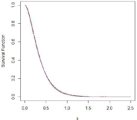
Plot of the survival functions of X1:2 (dashed line) and
3.4. Dependent samples with Archimedean structure
Recently, some efforts are made to investigate stochastic comparisons on order statistics of random variables with Archimedean copulas. See, for example, [6], [25], [24] and [14]. In this section we derive new result on the usual stochastic order between extreme order statistics of two heterogeneous random vectors with the dependent components having ES marginals and Archimedean copula structure. Specifically, by X ~ ES(α, λ, ϕ) we denote the sample having the Archimedean copula with generator ϕ and for i = 1,...,n, Xi ~ ES(αi, λ).
The largest order statistic Xn:n of the sample X ~ ES(α , λ, ϕ1) gets distribution function
Theorem 3.7.
For X ~ ES(α, λ, ϕ1) and X* ~ ES(α*, λ, ϕ2),
- (i)
if ϕ1 or ϕ2 is log-convex, and ψ2 ○ ϕ1 is super-additive, then
- (ii)
if ϕ1 or ϕ2 is log-concave, and ψ1 ○ ϕ2 is super-additive, then
Proof.
According to Equation (3.6), Xn:n and
- (i)
We only prove the case that ϕ1 is log-convex, and the other case can be finished similarly. First we show that J(α, λ, x, ϕ1) is decreasing and Schur-concave function of αi, i = 1,...,n. Since ϕ1 is decreasing, we have
That is, J(α, λ, x, ϕ1) is decreasing in αi for i = 1,...,n. Furthermore, for i ≠ j, the decreasing ϕ1 implies
whereThen Schur-concavity of J(α, λ, x, ϕ1) follows from Theorem 3.A.4. in [28]. According to Theorem 3.A.8 of [28], α ≽w α* implies J(α, λ, x, ϕ1) ≤ J(α*, λ, x, ϕ1). On the other hand, since ψ2 ○ ϕ1 is super-additive, by Lemma A.1. of [24], we have J(α*, λ, x, ϕ1) ≤ J(α*, λ, x, ϕ2). So, it holds that
That is,
- (ii)
We omit its proof due to the similarity to that of Part (i).
Note that Theorem 3.7 for particular case λ = 1 in [14] has been proved.
From Theorem 3.7 (i) and the fact that weak log-majorization implies weak submajorization, we readily obtain the following corollary.
Corollary 3.6.
For X ~ ES(α, λ, ϕ1) and X* ~ ES(α*, λ, ϕ2),
if ϕ1 or ϕ2 is log-convex, and ψ2 ○ ϕ1 is super-additive, then
Letting λ = 1 in Corollary 3.6 leads to the following corollary for PRH samples.
Corollary 3.7.
For X ~ PRH(α, ϕ1) and X* ~ PRH(α*, λ, ϕ2),
if ϕ1 or ϕ2 is log-convex, and ψ2 ○ ϕ1 is super-additive, then
Note that [14] in Theorem 5.2 proved the stochastic order between two largest order statistics when − log ϕ1 or − log ϕ2 is log-concave, but according to Corollary 3.7, we do not need to check the log-concavity of − log ϕ1 or − log ϕ2 and it is only enough that ϕ1 or ϕ2 be log-convex.
4. Conclusions
We used a new majorization notion, called f-majorization. The new majorization notion includes, as special cases, the usual majorization, the reciprocal majorization and the p-larger majorization notions. We provided a comprehensive account of the mathematical properties of the f-majorization order and gave applications of this order in the context of stochastic comparison of extreme order statistics.
Acknowledgement
We would like to express our deep appreciation to referees and Dr Javanshiri for their helpful comments that improved this paper.
References
Cite this article
TY  - JOUR
AU  - Esmaeil Bashkar
AU  - Hamzeh Torabi
AU  - Ali Dolati
AU  - Félix Belzunce
PY  - 2018
DA  - 2018/09/30
TI  - f-Majorization with Applications to Stochastic Comparison of Extreme Order Statistics
JO  - Journal of Statistical Theory and Applications
SP  - 520
EP  - 536
VL  - 17
IS  - 3
SN  - 2214-1766
UR  - https://doi.org/10.2991/jsta.2018.17.3.8
DO  - 10.2991/jsta.2018.17.3.8
ID  - Bashkar2018
ER  -